source_components

Tests for the functions in WODEN/src/source_components.cu. These functions calculate visibilities for the different COMPONENT types, as well as calling the various beam models to be applied to the visibilities.

test_apply_beam_gains.c

This calls source_components::test_kern_apply_beam_gains, which tests source_components::kern_apply_beam_gains. This kernel applies beam gain and leakage terms to Stokes visibilities to create linear Stokes polarisation visibilities via:

\[\begin{split}\begin{eqnarray} \mathrm{V}^{XX}_{12} = (g_{1x}g_{2x}^{\ast} + D_{1x}D_{2x}^{\ast})\mathrm{V}^{I}_{12} + (g_{1x}g_{2x}^{\ast} - D_{1x}D_{2x}^{\ast})\mathrm{V}^{Q}_{12} \\ + (g_{1x}D_{2x}^{\ast} + D_{1x}g_{2x}^{\ast})\mathrm{V}^{U}_{12} + i(g_{1x}D_{2x}^{\ast} - D_{1x}g_{2x}^{\ast})\mathrm{V}^{V}_{12} \end{eqnarray}\end{split}\]

\[\begin{split}\begin{eqnarray} \mathrm{V}^{XY}_{12} = (g_{1x}D_{2y}^{\ast} + D_{1x}g_{2y}^{\ast})\mathrm{V}^{I}_{12} + (g_{1x}D_{2y}^{\ast} - D_{1x}g_{2y}^{\ast})\mathrm{V}^{Q}_{12} \\ + (g_{1x}g_{2y}^{\ast} + D_{1x}D_{2y}^{\ast})\mathrm{V}^{U}_{12} + i(g_{1x}g_{2y}^{\ast} - D_{1x}D_{2y}^{\ast})\mathrm{V}^{V}_{12} \end{eqnarray}\end{split}\]

\[\begin{split}\begin{eqnarray} \mathrm{V}^{XY}_{12} = (g_{1x}D_{2y}^{\ast} + D_{1x}g_{2y}^{\ast})\mathrm{V}^{I}_{12} + (g_{1x}D_{2y}^{\ast} - D_{1x}g_{2y}^{\ast})\mathrm{V}^{Q}_{12} \\ + (g_{1x}g_{2y}^{\ast} + D_{1x}D_{2y}^{\ast})\mathrm{V}^{U}_{12} + i(g_{1x}g_{2y}^{\ast} - D_{1x}D_{2y}^{\ast})\mathrm{V}^{V}_{12} \end{eqnarray}\end{split}\]

\[\begin{split}\begin{eqnarray} \mathrm{V}^{YY}_{12} = (D_{1y}D_{2y}^{\ast} + g_{1y}g_{2y}^{\ast})\mathrm{V}^{I}_{12} + (D_{1y}D_{2y}^{\ast} - g_{1y}g_{2y}^{\ast})\mathrm{V}^{Q}_{12} \\ + (D_{1y}g_{2y}^{\ast} + g_{1y}D_{2y}^{\ast})\mathrm{V}^{U}_{12} + i(D_{1y}g_{2y}^{\ast} - g_{1y}D_{2y}^{\ast})\mathrm{V}^{V}_{12} \end{eqnarray}\end{split}\]

where \(\ast\) means complex conjugate, \(g_x, D_x, D_y, g_y\) are beam gain and leakage terms, with subscript 1 and 2 meaning antenna 1 and 2, and \(\mathrm{V}^I, \mathrm{V}^Q, \mathrm{V}^U, \mathrm{V}^V\) the Stokes visibilities. These tests try a number of combinations of values that have a simple outcome, and tests that the function returns the expected values. The combinations are shown in the table below. For all combinations, the beam gain and leakage is used for both antennas in the above equations. Each entry is a complex values and should be read as real,imag. Both FLOAT and DOUBLE code are just tested to a 32 bit accuracy here as these a simple numbers that require little precision.

\(g_x\)	\(D_x\)	\(D_y\)	\(g_y\)	\(\mathrm{V}^I\)	\(\mathrm{V}^Q\)	\(\mathrm{V}^U\)	\(\mathrm{V}^V\)	\(\mathrm{V}^{XX}\)	\(\mathrm{V}^{XY}\)	\(\mathrm{V}^{YX}\)	\(\mathrm{V}^{YY}\)
1,0	0,0	0,0	1,0	1,0	0,0	0,0	0,0	1,0	0,0	0,0	1,0
1,0	0,0	0,0	1,0	0,0	1,0	0,0	0,0	1,0	0,0	0,0	-1,0
1,0	0,0	0,0	1,0	0,0	0,0	1,0	0,0	0,0	1,0	1,0	0,0
1,0	0,0	0,0	1,0	0,0	0,0	0,0	1,0	0,0	0,1	0,-1	0,0
0,0	1,0	1,0	0,0	1,0	0,0	0,0	0,0	1,0	0,0	0,0	1,0
0,0	1,0	1,0	0,0	0,0	1,0	0,0	0,0	-1,0	0,0	0,0	1,0
0,0	1,0	1,0	0,0	0,0	0,0	1,0	0,0	0,0	1,0	1,0	0,0
0,0	1,0	1,0	0,0	0,0	0,0	0,0	1,0	0,0	0,-1	0,1	0,0
2,0	2,0	2,0	2,0	1,0	0,0	0,0	0,0	8,0	8,0	8,0	8,0
2,0	2,0	2,0	2,0	0,0	1,0	0,0	0,0	0,0	0,0	0,0	0,0
2,0	2,0	2,0	2,0	0,0	0,0	1,0	0,0	8,0	8,0	8,0	8,0
2,0	2,0	2,0	2,0	0,0	0,0	0,0	1,0	0,0	0,0	0,0	0,0
1,2	3,4	5,6	7,8	1,0	0,0	0,0	0,0	30,0	70,8	70,-8	174,0
1,2	3,4	5,6	7,8	0,0	1,0	0,0	0,0	-20,0	-36,0	-36,0	-52,0
1,2	3,4	5,6	7,8	0,0	0,0	1,0	0,0	22,0	62,8	62,-8	166,0
1,2	3,4	5,6	7,8	0,0	0,0	0,0	1,0	-4,0	-4,-16	-4,16	-4,0

test_calc_measurement_equation.c

This calls source_components::test_kern_calc_measurement_equation, which calls source_components::kern_calc_measurement_equation, which in turn is testing the device code source_components::calc_measurement_equation (which is used internally in WODEN in another kernel that calls multiple device functions, so I had to write a new kernel to test it alone.)

The following methodology is also written up the JOSS paper (TODO link JOSS paper once it’s accepted), where it’s used in a sky model + array layout through to visibility end-to-end version. Here we directly test the fuction above.

calc_measurement_equation calculates the phase-tracking measurement equation:

\[V(u,v,w) = \exp \left[ 2\pi i\left( ul + vm + w(n-1) \right) \right]\]

We can use Euler’s formula to split this into real and imaginary components. If I label the phase for a particular source and baseline as

\[\phi = 2\pi \left( ul + vm + w(n-1)\right)\]

then the real and imaginary parts of the visibility \(V_{re}\), \(V_{im}\) are

\[\begin{split}V_{re} = \cos(\phi) \\ V_{im} = \sin(\phi)\end{split}\]

A definitive test of the calc_measurement_equation function then is to then set \(\phi\) to a number of values which produce known sine and cosine outputs, by selecting specific combinations of u,v,w and l,m,n. First of all, consider the case when u,v,w = 1,1,1. In that case,

\[\frac{\phi_{\mathrm{simple}}}{2\pi} = l + m + (n-1).\]

if we further set l == m, we end up with

\[\begin{split}\frac{\phi_{\mathrm{simple}}}{2\pi} = 2l + (n-1), \\ l = \sqrt{\left( \frac{1 - n^2}{2} \right)}\end{split}\]

I shoved those two equations into Wolfram Alpha who assured me that a solution for n here is

\[n = \frac{\sqrt{2}\sqrt{-\phi_{\mathrm{simple}}^2 - 4\pi\phi_{\mathrm{simple}} + 8\pi^2} + \phi_{\mathrm{simple}} + 2\pi}{6\pi}\]

which we can then use to calculate values for l,m through

\[l = m = \sqrt{\frac{1 - n^2}{2}}.\]

By selecting the following values for \(\phi\), we can create the following set of l,m,n coords, which have the a known set of outcomes:

\(\phi_{\mathrm{simple}}\)	l,m	n	\(\cos(\phi)\)	\(\sin(\phi)\)
\(0\)	0.0	1.0	\(1.0\)	\(0\)
\(\pi/6\)	0.0425737516338956	0.9981858300655398	\(\sqrt{3}/2\)	\(0.5\)
\(\pi/4\)	0.0645903244635131	0.9958193510729726	\(\sqrt{2}/2\)	\(\sqrt{2}/2\)
\(\pi/3\)	0.0871449863555500	0.9923766939555675	\(0.5\)	\(\sqrt{3}/2\)
\(\pi/2\)	0.1340695840364469	0.9818608319271057	\(0.0\)	\(1.0\)
\(2\pi/3\)	0.1838657911209207	0.9656017510914922	\(-0.5\)	\(\sqrt{3}/2\)
\(3\pi/4\)	0.2100755148372292	0.9548489703255412	\(-\sqrt{2}/2\)	\(\sqrt{2}/2\)
\(5\pi/6\)	0.2373397982598921	0.9419870701468823	\(-\sqrt{3}/2\)	\(0.5\)
\(\pi\)	0.2958758547680685	0.9082482904638630	\(-1.0\)	\(0.0\)
\(7\pi/6\)	0.3622725654470420	0.8587882024392495	\(-\sqrt{3}/2\)	\(-0.5\)
\(5\pi/4\)	0.4003681253515569	0.8242637492968862	\(-\sqrt{2}/2\)	\(-\sqrt{2}/2\)

Note

If you try and go higher in \(\phi\) then because I set \(l == m\) you no longer honour \(\sqrt{l^2 + m^2 + n^2} <= 1.0\) I think this range of angles is good enough coverage though.

This is a great test for when \(u,v,w = 1\), but we want to test a range of baseline lengths to check our function is consistent for short and long baselines. We can play another trick, and set all baseline coords to be equal, i.e. \(u = v = w = b\) where \(b\) is baseline length. In this form, the phase including the baseline length \(\phi_{b}\) is

\[\phi_{b} = 2\pi b\left( l + m + n - 1 \right) = b\phi_{\mathrm{simple}}.\]

As sine/cosine are periodic functions, the following is true:

\[\phi_{\mathrm{simple}} = \phi_{\mathrm{simple}} + 2\pi \mathrm{n}\]

where \(\mathrm{n}\) is some integer. This means for a given \(\phi_{\mathrm{simple}}\) from the table above, we can find an appropriate \(b\) that should still result in the expected sine and cosine outputs by setting

\[\begin{split}b\phi_{\mathrm{simple}} = \phi_{\mathrm{simple}} + 2\pi \mathrm{n} \\ b = \frac{\phi_{\mathrm{simple}} + 2\pi \mathrm{n}}{\phi_{\mathrm{simple}}}\end{split}\]

for a range of \(\mathrm{n}\) values. The values of \(\mathrm{n}\) and the resultant size of \(b\) that I use in testing are shown in the table below (note for \(\phi_{\mathrm{simple}} = 0\) I just set \(b = 2\pi \mathrm{n}\) as the effects of \(l,m,n\) should set everything to zero regardless of baseline coords).

\(\phi_{\mathrm{simple}}\)	\(b(\mathrm{n=0})\)	\(b(\mathrm{n=1})\)	\(b(\mathrm{n=10})\)	\(b(\mathrm{n=100})\)	\(b(\mathrm{n=1000})\)	\(b(\mathrm{n=10000})\)
\(0\)	0.0	6.3	62.8	628.3	6283.2	62831.9
\(\pi/6\)	1.0	13.0	121.0	1201.0	12001.0	120001.0
\(\pi/4\)	1.0	9.0	81.0	801.0	8001.0	80001.0
\(\pi/3\)	1.0	7.0	61.0	601.0	6001.0	60001.0
\(\pi/2\)	1.0	5.0	41.0	401.0	4001.0	40001.0
\(2\pi/3\)	1.0	4.0	31.0	301.0	3001.0	30001.0
\(3\pi/4\)	1.0	3.7	27.7	267.7	2667.7	26667.7
\(5\pi/6\)	1.0	3.4	25.0	241.0	2401.0	24001.0
\(\pi\)	1.0	3.0	21.0	201.0	2001.0	20001.0
\(7\pi/6\)	1.0	2.7	18.1	172.4	1715.3	17143.9
\(5\pi/4\)	1.0	2.6	17.0	161.0	1601.0	16001.0

This gives a range of baseline lengths from 1 to \(> 10^4\) wavelengths.

In this test, I run every combination of \(l,m,n\) and \(u,v,w = b\) for each \(\phi_{\mathrm{simple}}\) from the tables above, and assert that the real and imaginary of every output visibility match the expected values of \(\sin(\phi_{\mathrm{simple}})\) and \(\cos(\phi_{\mathrm{simple}})\). When compiling with FLOAT precision, I assert the outputs must be within an absolute tolerance of 2e-3, and for DOUBLE a tolerance of 2e-9.

The error scales with the length of baseline, as shown in this plot below. Here, I have plotted the fractional offset of the recovered value of \(\sin(\phi_{\mathrm{simple}})\) (imaginary part of the visibility) and \(\cos(\phi_{\mathrm{simple}})\) (real part of the visibility), compared to their analytically expected outcome. I’ve plotted each \(\phi_{\mathrm{simple}}\) as a different symbol, with the FLOAT in blue and DOUBLE in orange.

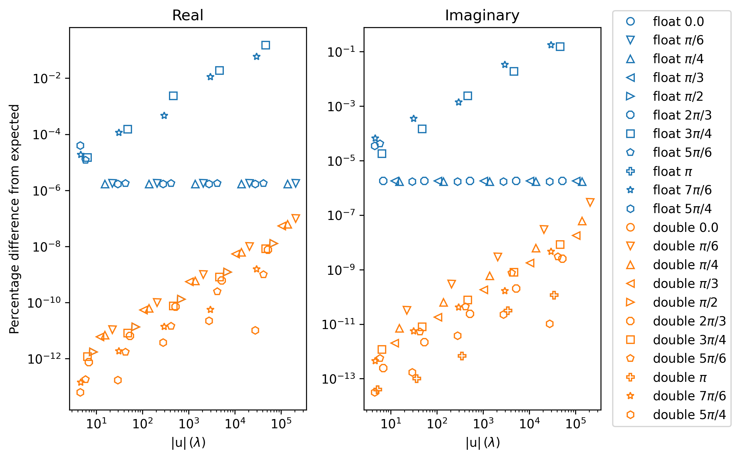
You can see as you increase baseline length, a general trend of increasing error is seen. Note these are the absolute differences plotted here, to work on a log10 scale. For the DOUBLE results, it’s close to 50% a negative or positive offset from expected. The FLOAT results that perform the worst (where \(\phi_{\mathrm{simple}} = 3\pi/4,\, 7\pi/6\)) correspond to values of \(b\) with large fractional values (see the table above), showing how the 32 bit precision fails to truthfully report large fractional numbers.

As a second test, I setup 10,000 u,v,w ranging from -1000 to 1000 wavelengths, and 3600 l,m,n coordinates that span the entire sky, and run them through source_components::test_kern_calc_measurement_equation and check they equal the equivalent measurement equation as calculated by C in 64 bit precisions. This checks the kernel works for a range of input coordinates. I assert the CUDA outputs must be within an absolute tolerance of 1e-7 for the FLOAT code, and 1e-15 for the DOUBLE code.

test_extrap_stokes.c

This calls source_components::test_kern_extrap_stokes, which calls source_components::kern_extrap_stokes, which handles extrapolating a reference flux density to a number of frequencies, given a spectral index.

Five test cases are used, with the following parameters:

Reference Freq (MHz)	Spectral Index	Stokes I	Stokes Q	Stokes U	Stokes V
50	0.0	1.0	0.0	0.0	0.0
100	-0.8	1.0	0.0	0.0	0.0
150	0.5	1.0	1.0	0.0	0.0
200	-0.5	1.0	0.0	1.0	0.0
250	1.0	1.0	0.0	0.0	1.0

Each of these test cases is extrapolated to 50, 100, 150, 200, 250 MHz. The CUDA outputs are testing as being equal to

\[S_{\mathrm{extrap}} = S_{\mathrm{ref}} \left( \frac{\nu_{\mathrm{ref}}}{\nu_{\mathrm{extrap}}} \right)^{\alpha}\]

as calculated in 64 bit precision in C code in test_extrap_stokes.c. The FLOAT complied code must match the C estimate to within an absolute tolerance of 1e-7, and a tolerance of 1e-15 for the DOUBLE compiled code.

test_get_beam_gains.c

This calls source_components::test_kern_get_beam_gains, which calls source_components::kern_get_beam_gains, which in turn is testing the device code source_components::get_beam_gains. This function handles grabbing the pre-calculated beam gains for a specific beam model, time, and frequency (assuming the beam gains have already been calculated). kern_get_beam_gains is setup to call get_beam_gains for multiple inputs and recover them into a set of output arrays.

Beam gain calculations are stored in primay_beam_J* arrays, including all frequency and time steps, as well as all directions on the sky. This test sets all real entries in the four primay_beam_J* beam gain arrays to the value of their index. In this way, we can easily predict the expected value in the outputs as being the index of the beam gain we wanted to select. I’ve set the imaginary to zero.

This test runs with two time steps, two frequency steps, three baselines, and four beam models. Three different outcomes are expected given the beam model:

• ANALY_DIPOLE, GAUSS_BEAM: The values of the gains are tested to match the expected index. The leakage terms are tested to be zero as the models have no leakage terms

• FEE_BEAM, FEE_BEAM_INTERP, MWA_ANALY: Both the beam gain and leakage terms are tested as these models include leakage terms

• NO_BEAM: The gain terms are tested to be 1.0, and leakage to be 0.0

Both FLOAT and DOUBLE code are tested to a 32 bit accuracy here as these are simple numbers that require little precision.

test_source_component_common.c

This calls source_components::test_source_component_common, which calls source_components::source_component_common. source_component_common is run by all visibility calculation functions (the functions kern_calc_visi_point, kern_calc_visi_gauss, kern_calc_visi_shape). It handles calculating the l,m,n coordinates and beam response for all COMPONENTs in a sky model, regardless of the type of COMPONENT.

Similarly to the tests in test_lmn_coords.c, I setup a slice of 9 RA coordinates, and hold the Dec constant, set the phase centre to RA\(_{\textrm{phase}}\), Dec\(_{\textrm{phase}}\) = \(0^\circ, 0^\circ\). This way I can analytically predict what the l,m,n calculated coordinates should be (which are tested to be within 1e-15 of expected values).

In these tests I run with three time steps, two frequency steps (100 and 200 MHz), and five baselines (the coordinates of which don’t matter, but change the size of the outputs, so good to have a non-one value). I input a set of az,za coords that match the RA,Dec coords for an LST = 0.0. As I have other tests that check the sky moves with time, I just set the sky to be stationary with time here, to keep the test clean.

For each primary beam type, I run the 9 COMPONENTs through the test, and check the calcualted l,m,n are correct, and check that the calculated beam values match a set of expected values, which are stored in test_source_component_common.h. As with previous tests varying the primary beam, I check that leakage terms should be zero when the model doesn’t include them.

The absolute tolerance values used for the different beam models, for the two different precisions are shown in the table below. Note I’ve only stored the expected values for some of the beams to 1e-7 accuracy, as the absolute accuracy of these functions beam functions is tested elsewhere. The GAUSS_BEAM values are calculated analytically in the same test as described in test_gaussian_beam.c.

Beam type	FLOAT tolerance	DOUBLE tolerance
GAUSS_BEAM	1e-7	1e-12
ANALY_DIPOLE	1e-6	1e-7
FEE_BEAM	3e-2	1e-7
FEE_BEAM_INTERP	3e-2	1e-7
MWA_ANALY	1e-7	1e-12

test_kern_calc_visi_point.c

This calls source_components::test_kern_calc_visi_point, which calls source_components::kern_calc_visi_point. This kernel calculates the visibility response for POINT COMPONENTs for a number of sky directions, for all time and frequency steps, and all baselines.

I set up a grid of 25 l,m coords with l,m coords ranging over -0.5, -0.25, 0.0, 0.25, 0.5. I run a simulation with 10 baselines, where I set u,v,w to:

\[\begin{split}u,v = 100(b_{\mathrm{ind}} + 1) \\ w = 10(b_{\mathrm{ind}} + 1)\end{split}\]

where \(b_{\mathrm{ind}}\) is the baseline index, meaning the test covers the baseline range \(100 < u,v <= 1000\) and \(10 < w <= 100\). The test also runs three frequncies, 150, 175, 200 MHz, and two time steps. As I am providing predefined u,v,w, I don’t need to worry about LST effects, but I simulate with two time steps to make sure the resultant visibilities end up in the right order.

Overall, I run three groups of tests here:

• Keeping the beam gains and flux densities constant at 1.0

• Varying the flux densities with frequency and keeping the beam gains constant at 1.0. When varying the flux, I set the Stokes I flux of each component to it’s index + 1, so we end up with a range of fluxes between 1 and 25. I set the spectral index to -0.8.

• Varying the beam gains with frequency and keeping the flux densities constant at 1.0. As the beam can vary with time, frequency, and direction on sky, I assign each beam gain a different value. As num_freqs*num_times*num_components = 375, I set the real of all beam gains to \(\frac{1}{375}(B_{\mathrm{ind}} + 1)\), where \(B_{\mathrm{ind}}\) is the beam value index. This way we get a unique value between 0 and 1 for all beam gains, allowing us to test time/frequency is handled correctly by the function under test

Each set of tests is run for all six primary beam types, so a total of 18 tests are called. Each test calls kern_calc_visi_point, which should calculate the measurement equation for all baselines, time steps, frequency steps, and COMPONENTs. It should also sum over COMPONENTs to get the resultant visibility for each baseline, time, and freq. To test the outputs, I have created equivalent C functions at 64 bit precisions in test_kern_calc_visi_common.c to calculate the measurement equation for the given inputs. For all visibilities, for the FLOAT version I assert the CUDA code output must match the C code output to within an fractional tolerance of 1e-5 to the C value, for both the real and imaginary parts. For the DOUBLE code, the fractional tolerance is 1e-13. I’ve switched to fractional tolerance here as the range of magnitudes covered by these visibilities means a small absolute tolernace will fail a large magnitude visibility when it reports a value that is correct to 1e-11%.

test_kern_calc_visi_gauss.c

This calls source_components::test_kern_calc_visi_gauss, which calls source_components::kern_calc_visi_gauss. This kernel calculates the visibility response for GAUSSIAN COMPONENTs for a number of sky directions, for all time and frequency steps, and all baselines.

This runs all tests as described by test_kern_calc_visi_point.c, plus a fourth set of tests that varies the position angle, major, and minor axis of the input GAUSSIAN components, for a total of 24 tests. Again, I have C code to test the CUDA code against. I assert the CUDA code output must match the C code output to within an fractional tolerance of 1e-5 to the C value, for both the real and imaginary parts. For the DOUBLE code, the fractional tolerance is 1e-13.

test_kern_calc_visi_shape.c

This calls source_components::test_kern_calc_visi_gauss, which calls source_components::kern_calc_visi_gauss. This kernel calculates the visibility response for GAUSSIAN COMPONENTs for a number of sky directions, for all time and frequency steps, and all baselines.

This runs all tests as described by test_kern_calc_visi_gauss.c, plus a fifth set of tests that gives multiple shapelet basis function parameters to the input SHAPELET components, for a total of 30 tests. Again, I have C code to test the CUDA code against.

The final 5th test really pushes the FLOAT code hard, as the range of magnitudes of the visibilities is large. As a result, FLOAT code is tested to to within a fractional tolerance of 1e-2 to the C values (which happens mostly when the expected value is around 1e-5 Jy, so a fractional offset of 1e-2 is an absolute offset of 1e-7 Jy), for both the real and imaginary parts. For the DOUBLE code, the fractional tolerance is 1e-12.

test_update_sum_visis.c

This calls source_components::test_kern_update_sum_visis, which in turn calls source_components::kern_update_sum_visis. This kernel gathers pre-calculated primary beam values, unpolarised visibilities, Stokes flux densities, and combines them all into linear polarisation Stokes visibilities. It then sums all COMPONENTs together onto the final set of linear polarisation visibilities.

This code runs three sets of tests, each with three baselines, four time steps, three frequencies, and ten COMPONENTs. For each set of tests, the input arrays that are being tested have their values set to the index of the value, making the summation able to test whether the correct time, frequency, and beam indexes are being summed into the resultant visibilities. The three sets of tests consist of:

• Varying the beam gains, while keeping the flux densities and unpolarised measurement equations constant.

• Varying the flux densities, while keeping the beam gains and unpolarised measurement equations constant.

• Varying the unpolarised measurement equations, while keeping the beam gains and flux densities constant.

Each set of tests is run for all primary beam types, for a total of 18 tests. The different beam models have different expected values depending on whether they include leakage terms or not.