primary_beam_cuda

Tests for the functions in WODEN/src/primary_beam_cuda.cu. These functions calculate the beam responses for the EDA2 and Gaussian beam models.

test_gaussian_beam.c

This calls primary_beam_cuda::test_kern_gaussian_beam, which in turn tests primary_beam_cuda::kern_gaussian_beam, the kernel that calculates the Gaussian primary beam response. As a Gaussian is an easy function to calculate, I’ve setup tests that calculate a north-south and east-west strip of the beam response, and then compare that to a 1D Gaussian calculation.

As kern_gaussian_beam just takes in l,m coords, these tests just generate 100 l,m coords that span from -1 to +1. The tests check whether the kernel produces the expected coordinates in the l and m strips, as well as changing with frequency as expected, by testing 5 input frequencies with a given reference frequency. For each input frequency \(\nu\), the output is checked against the following calculations:

• When setting m = 0, assert gain = \(\exp\left[-\frac{1}{2} \left( \frac{l}{\sigma} \frac{\nu}{\nu_0} \right)^2 \right]\)

• When setting l = 0, assert gain = \(\exp\left[-\frac{1}{2} \left( \frac{m}{\sigma} \frac{\nu}{\nu_0} \right)^2 \right]\)

where \(\nu_0\) is the reference frequency, and \(\sigma_0\) the std of the Gaussian in terms of l,m coords. These calculations are made using C with 64 bit precision. The beam responses are tested to be within an absolute tolerance of 1e-10 from expectations for the FLOAT compiled code, and 1e-16 for the DOUBLE compiled code.

test_analytic_dipole_beam.c

This calls primary_beam_cuda::test_analytic_dipole_beam, which in turn tests primary_beam_cuda::calculate_analytic_dipole_beam, code that copies az/za angles into GPU memory, calculates an analytic dipole response toward those directions, and then frees the az/za coords from GPU memory.

Nothing exiting in this test, just call the function for 25 directions on the sky, for two time steps and two frequencies (a total of 100 beam calculations), and check that the real beam gains match stored expected values, and the imaginary values equal zero. The expected values have been generated using the DOUBLE precision compiled code, and so the absolute tolerance of within 1e-12 is set by how many decimal places I’ve stored in the lookup table. The FLOAT precision must match within 1e-6 of these stored values.

test_MWA_analytic.c

Todo

stick the maths of what the analytic beam does here (it is involved).

This calls primary_beam_cuda::test_calculate_MWA_analytic_beam, which calls primary_beam_cuda::calculate_MWA_analytic_beam, which calculates an analytic version of the MWA primary beam, based on ideal dipoles. This code calculates the primary beam response of the MWA using methods from RTS. The analytic beam is purely real.

This test runs with an off-zenith pointing, with a grid of 201 by 201 of az/za or two time steps, and two frequencies (150 and 200MHz). The az/za coords for both time steps are identical, but test whether the time/frequency ordering of the outputs are correct. The beam responses are tested to be within an absolute tolerance of 1e-6 from expectations for the FLOAT compiled code, and 1e-8 for the DOUBLE compiled code (the responses are only stored to 1e-8 precision for testing to save space on disk).

If you want to look at your outputs, you can run:

$ python plot_MWA_analytic.py

will will plot the real components of beam responses of both the MWA analytic beam (jones_MWA_analy_gains_nside201_t00_f150.000MHz.png):

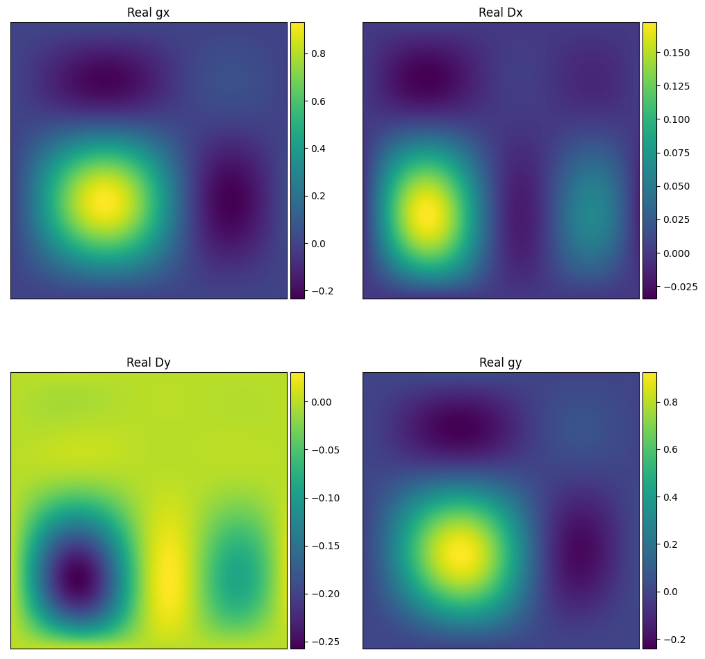
The testing here also runs comp_MWA_analytic_to_FEE.c, which runs the MWA FEE beam code for the same sky directions. This comparison is also plotted as (jones_MWA_analy_gains_nside201_t00_f150.000MHz.png):

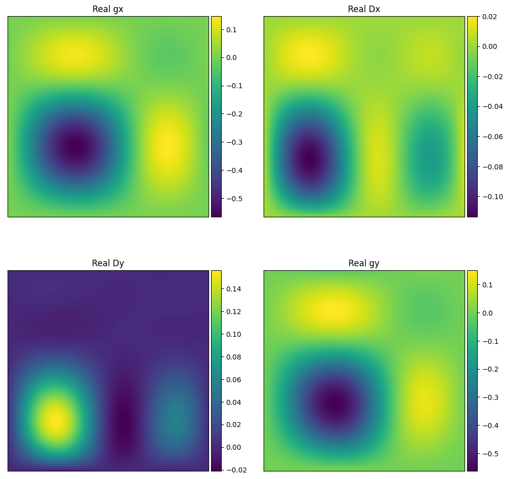
which gives us a sanity check that both beams point in the same direction for the same input az/za coords, and that they have similar structures on the sky, albeit they are negative of one another.

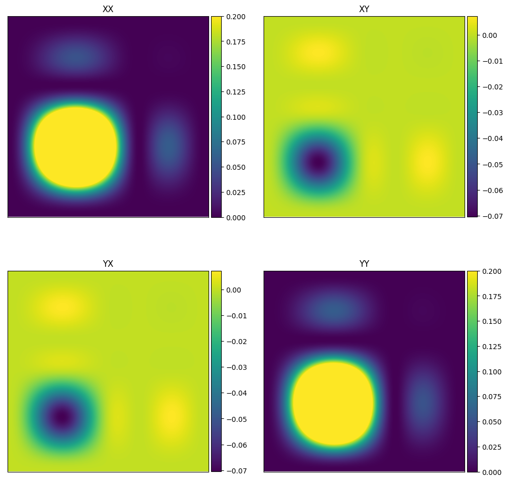
When we combine the gains and leakages to create linear Stokes, we see that we get similar beams. First of all, here is the RTS MWA analytic linear_pol_MWA_analy_gains_nside201_t00_f150.000MHz.png:

Comparing that the MWA FEE beam linear_pol_MWA_FEE_gains_nside201_t00_f150.000MHz.png:

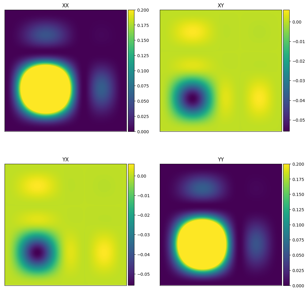
we see that all linear polarisations have the same signs and simliar structures.

The plotting script plots both frequencies and time steps for the analytic beam, letting you visually check that the outputs are ordered as expected.