EDA2 Haslam Map simulation

Note

Running the simulation and making all the images will take up around 1.8 GB storage.

In this simulation, we’ll use an all-sky healpix image with nside 256 (generated using pygdsm). For the sky model, I have converted every healpixel into a point source. You’ll need to download the skymodel from this googledoc link to pygsm_woden-list_100MHz_n256.txt and put it in the correct directory. If you’re comfortable with wget you can do:

$ cd WODEN/examples/EDA2_haslam
$ wget 'https://docs.google.com/uc?export=download&id=1TEELux33UClRTiZBFOzGJHF-XbLnZjUV' -O pygsm_woden-list_100MHz_n256.txt

To run the command, do:

$ ./EDA2_haslam_simulation.sh

which took 2 hours 11 mins on my machine (this is running in DOUBLE precision, it takes 1 hour 15 mins at FLOAT precision). This simulates 393,216 point sources for an array of 255 antennas. The command run is:

run_woden.py \
  --ra0=74.79589467 --dec0=-27.0 \
  --time_res=10.0 --num_time_steps=10 \
  --freq_res=10e+3 --coarse_band_width=10e+4 \
  --lowest_channel_freq=100e+6 \
  --cat_filename=pygsm_woden-list_100MHz_n256.txt \
  --array_layout=../../test_installation/array_layouts/EDA2_layout_255.txt \
  --date=2020-02-01T12:27:45.900 \
  --output_uvfits_prepend=./data/EDA2_haslam \
  --primary_beam=EDA2 \
  --sky_crop_components \
  --band_nums=1,2,3,4,5

Here is a line by line explanation of the command.

--ra0=74.79589467 --dec0=-27.0

sets the phase centre of the simulation.

--time_res=10.0 --num_time_steps=10

means there will be 10 time samples with 10 seconds between each sample.

--freq_res=10e+3 --coarse_band_width=10e+4 \
--lowest_channel_freq=100e+6 --band_nums=1,2,3,4,5

this combination of arguments will create 5 uvfits file outputs, each containing 10 frequency channels of width 10 kHz. The lowest band will start at 100 MHz, giving a total frequency coverage from 100 MHz to 100.5 MHz.

--cat_filename=pygsm_woden-list_100MHz_n256.txt

points towards the sky model.

--array_layout=../../test_installation/array_layouts/EDA2_layout_255.txt

points towrads an array file that contains local east, north, height coordinates (in metres). This is used in conjunction with latitude to generate baseline coordinates. The default --latitude is set to the MWA which is right next to the EDA2 so good enough for the example.

-date=2020-02-01T12:27:45.900

sets a UTC date which is used in conjunction with --longitude to calculate the LST (again, defaults to MWA which is good for purpose here).

--output_uvfits_prepend=./data/EDA2_haslam

sets the naming convention for the outputs, in conjunction with --band_nums=1,2,3,4,5 will produce the outputs:

./data/EDA2_haslam_band01.uvfits
./data/EDA2_haslam_band02.uvfits
./data/EDA2_haslam_band03.uvfits
./data/EDA2_haslam_band04.uvfits
./data/EDA2_haslam_band05.uvfits

--primary_beam=EDA2

selects the EDA2 primary beam.

--sky_crop_components

this means that sky model is cropped by COMPONENT and not by SOURCE. This model has the diffuse sky as a single SOURCE, so some COMPONENT s are always below the horizon so need this flag to not crop the whole sky out.

Note

The real EDA2 instrument has 256 antennas. CASA only allows a maximum of 255 elements in an array table, so imaging becomes a nightmare. For this example, to make an image, I’ve just left out an antenna to make my life easier.

Once you’ve run that, you can make an image via:

$ ./EDA2_haslam_imaging.sh

and you’ll see this:

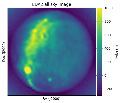
where we can see that the EDA2 can see essentially the whole sky, albeit at poor resolution.