source_components

Tests for the functions in src/source_components_common.c, src/source_components_cpu.c and src/source_components_gpu.cpp These functions run calculations common to all COMPONENT types, namely calculating lmn coordinates, extrapolating Stokes flux densities, calculating primary beam gains, visibility calculations, and calculating auto-correlations.

As always, all CPU and GPU functions are run through the same tests to ensure consistency between the two.

test_apply_beam_gains*.c

This calls source_components_gpu.cpp::kern_apply_beam_gains or source_components_cpu.c::apply_beam_gains_arrays_cpu. These functions apply beam gain and leakage terms to Stokes visibilities to create linear Stokes polarisation visibilities via:

\[\begin{split}\begin{eqnarray} \mathrm{V}^{XX}_{12} = (g_{1x}g_{2x}^{\ast} + D_{1x}D_{2x}^{\ast})\mathrm{V}^{I}_{12} + (g_{1x}g_{2x}^{\ast} - D_{1x}D_{2x}^{\ast})\mathrm{V}^{Q}_{12} \\ + (g_{1x}D_{2x}^{\ast} + D_{1x}g_{2x}^{\ast})\mathrm{V}^{U}_{12} + i(g_{1x}D_{2x}^{\ast} - D_{1x}g_{2x}^{\ast})\mathrm{V}^{V}_{12} \end{eqnarray}\end{split}\]

\[\begin{split}\begin{eqnarray} \mathrm{V}^{XY}_{12} = (g_{1x}D_{2y}^{\ast} + D_{1x}g_{2y}^{\ast})\mathrm{V}^{I}_{12} + (g_{1x}D_{2y}^{\ast} - D_{1x}g_{2y}^{\ast})\mathrm{V}^{Q}_{12} \\ + (g_{1x}g_{2y}^{\ast} + D_{1x}D_{2y}^{\ast})\mathrm{V}^{U}_{12} + i(g_{1x}g_{2y}^{\ast} - D_{1x}D_{2y}^{\ast})\mathrm{V}^{V}_{12} \end{eqnarray}\end{split}\]

\[\begin{split}\begin{eqnarray} \mathrm{V}^{XY}_{12} = (g_{1x}D_{2y}^{\ast} + D_{1x}g_{2y}^{\ast})\mathrm{V}^{I}_{12} + (g_{1x}D_{2y}^{\ast} - D_{1x}g_{2y}^{\ast})\mathrm{V}^{Q}_{12} \\ + (g_{1x}g_{2y}^{\ast} + D_{1x}D_{2y}^{\ast})\mathrm{V}^{U}_{12} + i(g_{1x}g_{2y}^{\ast} - D_{1x}D_{2y}^{\ast})\mathrm{V}^{V}_{12} \end{eqnarray}\end{split}\]

\[\begin{split}\begin{eqnarray} \mathrm{V}^{YY}_{12} = (D_{1y}D_{2y}^{\ast} + g_{1y}g_{2y}^{\ast})\mathrm{V}^{I}_{12} + (D_{1y}D_{2y}^{\ast} - g_{1y}g_{2y}^{\ast})\mathrm{V}^{Q}_{12} \\ + (D_{1y}g_{2y}^{\ast} + g_{1y}D_{2y}^{\ast})\mathrm{V}^{U}_{12} + i(D_{1y}g_{2y}^{\ast} - g_{1y}D_{2y}^{\ast})\mathrm{V}^{V}_{12} \end{eqnarray}\end{split}\]

where \(\ast\) means complex conjugate, \(g_x, D_x, D_y, g_y\) are beam gain and leakage terms, with subscript 1 and 2 meaning antenna 1 and 2, and \(\mathrm{V}^I, \mathrm{V}^Q, \mathrm{V}^U, \mathrm{V}^V\) the Stokes visibilities. These tests try a number of combinations of values that have a simple outcome, and tests that the function returns the expected values. The combinations are shown in the table below. For all combinations, the beam gain and leakage is used for both antennas in the above equations. Each entry is a complex values and should be read as real,imag. Both FLOAT and DOUBLE code are just tested to a 32 bit accuracy here as these a simple numbers that require little precision.

\(g_x\)	\(D_x\)	\(D_y\)	\(g_y\)	\(\mathrm{V}^I\)	\(\mathrm{V}^Q\)	\(\mathrm{V}^U\)	\(\mathrm{V}^V\)	\(\mathrm{V}^{XX}\)	\(\mathrm{V}^{XY}\)	\(\mathrm{V}^{YX}\)	\(\mathrm{V}^{YY}\)
1,0	0,0	0,0	1,0	1,0	0,0	0,0	0,0	1,0	0,0	0,0	1,0
1,0	0,0	0,0	1,0	0,0	1,0	0,0	0,0	1,0	0,0	0,0	-1,0
1,0	0,0	0,0	1,0	0,0	0,0	1,0	0,0	0,0	1,0	1,0	0,0
1,0	0,0	0,0	1,0	0,0	0,0	0,0	1,0	0,0	0,1	0,-1	0,0
0,0	1,0	1,0	0,0	1,0	0,0	0,0	0,0	1,0	0,0	0,0	1,0
0,0	1,0	1,0	0,0	0,0	1,0	0,0	0,0	-1,0	0,0	0,0	1,0
0,0	1,0	1,0	0,0	0,0	0,0	1,0	0,0	0,0	1,0	1,0	0,0
0,0	1,0	1,0	0,0	0,0	0,0	0,0	1,0	0,0	0,-1	0,1	0,0
2,0	2,0	2,0	2,0	1,0	0,0	0,0	0,0	8,0	8,0	8,0	8,0
2,0	2,0	2,0	2,0	0,0	1,0	0,0	0,0	0,0	0,0	0,0	0,0
2,0	2,0	2,0	2,0	0,0	0,0	1,0	0,0	8,0	8,0	8,0	8,0
2,0	2,0	2,0	2,0	0,0	0,0	0,0	1,0	0,0	0,0	0,0	0,0
1,2	3,4	5,6	7,8	1,0	0,0	0,0	0,0	30,0	70,8	70,-8	174,0
1,2	3,4	5,6	7,8	0,0	1,0	0,0	0,0	-20,0	-36,0	-36,0	-52,0
1,2	3,4	5,6	7,8	0,0	0,0	1,0	0,0	22,0	62,8	62,-8	166,0
1,2	3,4	5,6	7,8	0,0	0,0	0,0	1,0	-4,0	-4,-16	-4,16	-4,0

test_calc_measurement_equation*.c

This calls source_components_gpu.cpp::kern_calc_measurement_equation or source_components_cpu.c::calc_measurement_equation_arrays_cpu. These functions calculate the phase-tracking measurement equation for a visibility, given the baseline coordinates and the source coordinates.

The following methodology is also written up in the JOSS WODEN paper where it’s used in a sky model + array layout through to visibility end-to-end version. Here we directly test the functions above.

calc_measurement_equation calculates the phase-tracking measurement equation:

\[V(u,v,w) = \exp \left[ 2\pi i\left( ul + vm + w(n-1) \right) \right]\]

We can use Euler’s formula to split this into real and imaginary components. If I label the phase for a particular source and baseline as

\[\phi = 2\pi \left( ul + vm + w(n-1)\right)\]

then the real and imaginary parts of the visibility \(V_{re}\), \(V_{im}\) are

\[\begin{split}V_{re} = \cos(\phi) \\ V_{im} = \sin(\phi)\end{split}\]

A definitive test of the calc_measurement_equation function then is to then set \(\phi\) to a number of values which produce known sine and cosine outputs, by selecting specific combinations of u,v,w and l,m,n. First of all, consider the case when u,v,w = 1,1,1. In that case,

\[\frac{\phi_{\mathrm{simple}}}{2\pi} = l + m + (n-1).\]

if we further set l == m, we end up with

\[\begin{split}\frac{\phi_{\mathrm{simple}}}{2\pi} = 2l + (n-1), \\ l = \sqrt{\left( \frac{1 - n^2}{2} \right)}\end{split}\]

I shoved those two equations into Wolfram Alpha who assured me that a solution for n here is

\[n = \frac{\sqrt{2}\sqrt{-\phi_{\mathrm{simple}}^2 - 4\pi\phi_{\mathrm{simple}} + 8\pi^2} + \phi_{\mathrm{simple}} + 2\pi}{6\pi}\]

which we can then use to calculate values for l,m through

\[l = m = \sqrt{\frac{1 - n^2}{2}}.\]

By selecting the following values for \(\phi\), we can create the following set of l,m,n coords, which have the a known set of outcomes:

\(\phi_{\mathrm{simple}}\)	l,m	n	\(\cos(\phi)\)	\(\sin(\phi)\)
\(0\)	0.0	1.0	\(1.0\)	\(0\)
\(\pi/6\)	0.0425737516338956	0.9981858300655398	\(\sqrt{3}/2\)	\(0.5\)
\(\pi/4\)	0.0645903244635131	0.9958193510729726	\(\sqrt{2}/2\)	\(\sqrt{2}/2\)
\(\pi/3\)	0.0871449863555500	0.9923766939555675	\(0.5\)	\(\sqrt{3}/2\)
\(\pi/2\)	0.1340695840364469	0.9818608319271057	\(0.0\)	\(1.0\)
\(2\pi/3\)	0.1838657911209207	0.9656017510914922	\(-0.5\)	\(\sqrt{3}/2\)
\(3\pi/4\)	0.2100755148372292	0.9548489703255412	\(-\sqrt{2}/2\)	\(\sqrt{2}/2\)
\(5\pi/6\)	0.2373397982598921	0.9419870701468823	\(-\sqrt{3}/2\)	\(0.5\)
\(\pi\)	0.2958758547680685	0.9082482904638630	\(-1.0\)	\(0.0\)
\(7\pi/6\)	0.3622725654470420	0.8587882024392495	\(-\sqrt{3}/2\)	\(-0.5\)
\(5\pi/4\)	0.4003681253515569	0.8242637492968862	\(-\sqrt{2}/2\)	\(-\sqrt{2}/2\)

Note

If you try and go higher in \(\phi\) then because I set \(l == m\) you no longer honour \(\sqrt{l^2 + m^2 + n^2} <= 1.0\) I think this range of angles is good enough coverage though.

This is a great test for when \(u,v,w = 1\), but we want to test a range of baseline lengths to check our function is consistent for short and long baselines. We can play another trick, and set all baseline coords to be equal, i.e. \(u = v = w = b\) where \(b\) is baseline length. In this form, the phase including the baseline length \(\phi_{b}\) is

\[\phi_{b} = 2\pi b\left( l + m + n - 1 \right) = b\phi_{\mathrm{simple}}.\]

As sine/cosine are periodic functions, the following is true:

\[\phi_{\mathrm{simple}} = \phi_{\mathrm{simple}} + 2\pi \mathrm{n}\]

where \(\mathrm{n}\) is some integer. This means for a given \(\phi_{\mathrm{simple}}\) from the table above, we can find an appropriate \(b\) that should still result in the expected sine and cosine outputs by setting

\[\begin{split}b\phi_{\mathrm{simple}} = \phi_{\mathrm{simple}} + 2\pi \mathrm{n} \\ b = \frac{\phi_{\mathrm{simple}} + 2\pi \mathrm{n}}{\phi_{\mathrm{simple}}}\end{split}\]

for a range of \(\mathrm{n}\) values. The values of \(\mathrm{n}\) and the resultant size of \(b\) that I use in testing are shown in the table below (note for \(\phi_{\mathrm{simple}} = 0\) I just set \(b = 2\pi \mathrm{n}\) as the effects of \(l,m,n\) should set everything to zero regardless of baseline coords).

\(\phi_{\mathrm{simple}}\)	\(b(\mathrm{n=0})\)	\(b(\mathrm{n=1})\)	\(b(\mathrm{n=10})\)	\(b(\mathrm{n=100})\)	\(b(\mathrm{n=1000})\)	\(b(\mathrm{n=10000})\)
\(0\)	0.0	6.3	62.8	628.3	6283.2	62831.9
\(\pi/6\)	1.0	13.0	121.0	1201.0	12001.0	120001.0
\(\pi/4\)	1.0	9.0	81.0	801.0	8001.0	80001.0
\(\pi/3\)	1.0	7.0	61.0	601.0	6001.0	60001.0
\(\pi/2\)	1.0	5.0	41.0	401.0	4001.0	40001.0
\(2\pi/3\)	1.0	4.0	31.0	301.0	3001.0	30001.0
\(3\pi/4\)	1.0	3.7	27.7	267.7	2667.7	26667.7
\(5\pi/6\)	1.0	3.4	25.0	241.0	2401.0	24001.0
\(\pi\)	1.0	3.0	21.0	201.0	2001.0	20001.0
\(7\pi/6\)	1.0	2.7	18.1	172.4	1715.3	17143.9
\(5\pi/4\)	1.0	2.6	17.0	161.0	1601.0	16001.0

This gives a range of baseline lengths from 1 to \(> 10^4\) wavelengths.

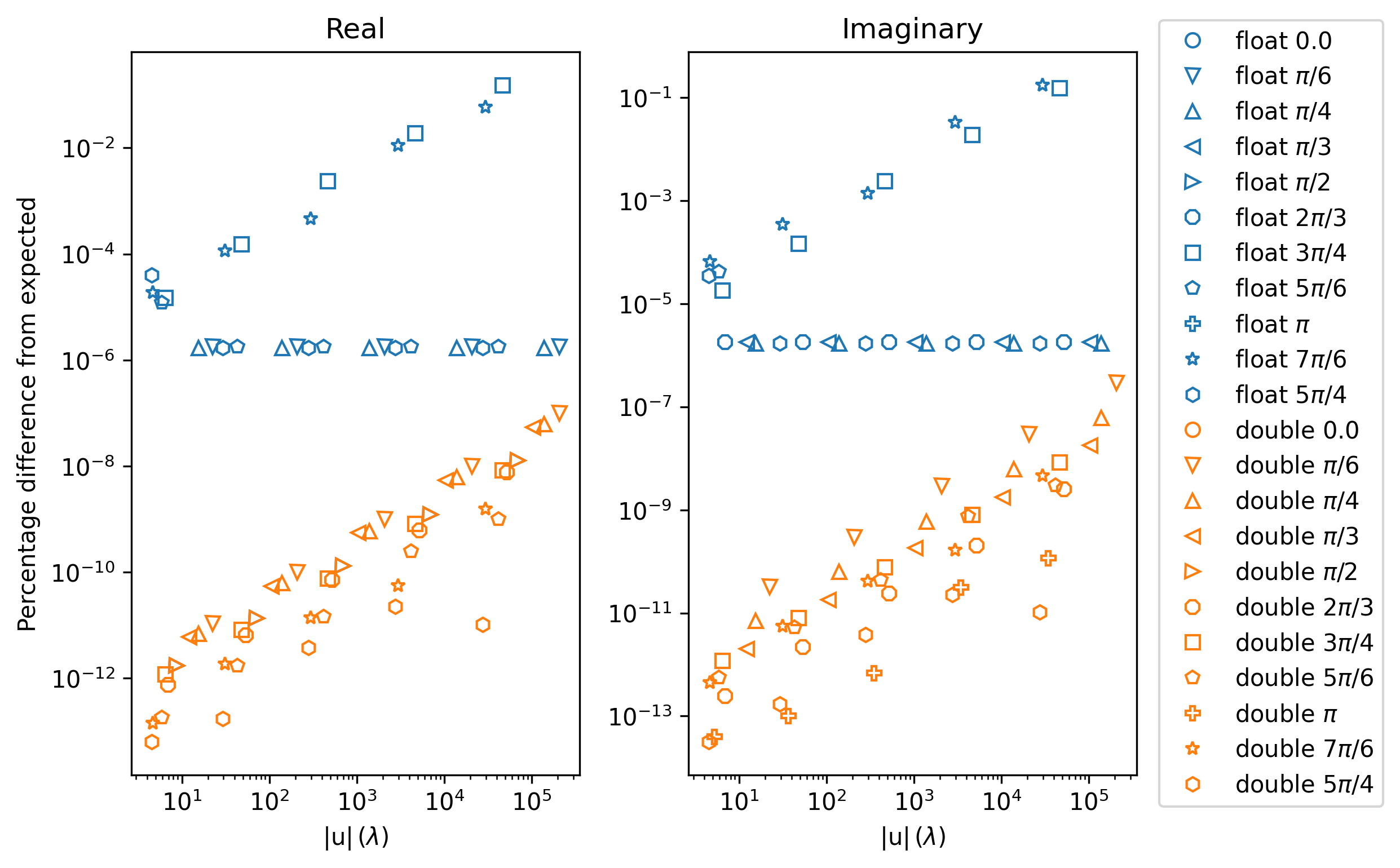
In this test, I run every combination of \(l,m,n\) and \(u,v,w = b\) for each \(\phi_{\mathrm{simple}}\) from the tables above, and assert that the real and imaginary of every output visibility match the expected values of \(\sin(\phi_{\mathrm{simple}})\) and \(\cos(\phi_{\mathrm{simple}})\). When compiling with FLOAT precision, I assert the outputs must be within an absolute tolerance of 2e-3, and for DOUBLE a tolerance of 2e-9.

The error scales with the length of baseline, as shown in this plot below. Here, I have plotted the fractional offset of the recovered value of \(\sin(\phi_{\mathrm{simple}})\) (imaginary part of the visibility) and \(\cos(\phi_{\mathrm{simple}})\) (real part of the visibility), compared to their analytically expected outcome. I’ve plotted each \(\phi_{\mathrm{simple}}\) as a different symbol, with the FLOAT in blue and DOUBLE in orange.

You can create this plot for yourself after running ctest via running python plot_measure_eq_results.py in cmake_testing/GPU_or_C_code/source_components.

You can see as you increase baseline length, a general trend of increasing error is seen. Note these are the absolute differences plotted here, to work on a log10 scale. For the DOUBLE results, it’s close to 50% a negative or positive offset from expected. The FLOAT results that perform the worst (where \(\phi_{\mathrm{simple}} = 3\pi/4,\, 7\pi/6\)) correspond to values of \(b\) with large fractional values (see the table above), showing how the 32 bit precision fails to truthfully report large fractional numbers.

As a second test, I setup 10,000 u,v,w ranging from -1000 to 1000 wavelengths, and 3600 l,m,n coordinates that span the entire sky, and run them through and check they equal the equivalent measurement equation as calculated by an equivalent test function.

test_extrap_stokes*.c

This calls source_components_common::extrapolate_Stokes, which calls many many different functions in source_components_cpu.c or source_components_gpu.cpp. extrapolate_Stokes handles extrapolating the flux density of component to a given set of frequencies. This covers all types of flux behaviours. Currently that POWER_LAW, CURVED_POWER_LAW, and LIST types for Stokes I, and POWER_LAW, CURVED_POWER_LAW, POLARISATION FRACTION, LIST, for linear and circular polarisation. Linear polarisation also has a P_LIST type, where a list of polarised fluxes are given, which are still used in conjunction with an RM. The LIST for linear polarisation requires two separate lists for Q and U.

Five components of each type of Stokes I flux behaviour are tested, each with randomly assigned values (these values are generated using the script WODEN/cmake_testing/source_components/write_test_extrap_stokes_header.py). For the LIST flux types, each list has a random number of entries, as well as each list entry begin given a random flux. Every component is also assigned random polarisation model for linear and circular polarisation.

The values are copied into a source_t struct, passed into functions being tested, and extrapolated to 100 frequencies between 50 and 300 MHz. The outputs are tested against equivalent C functions in double precision.

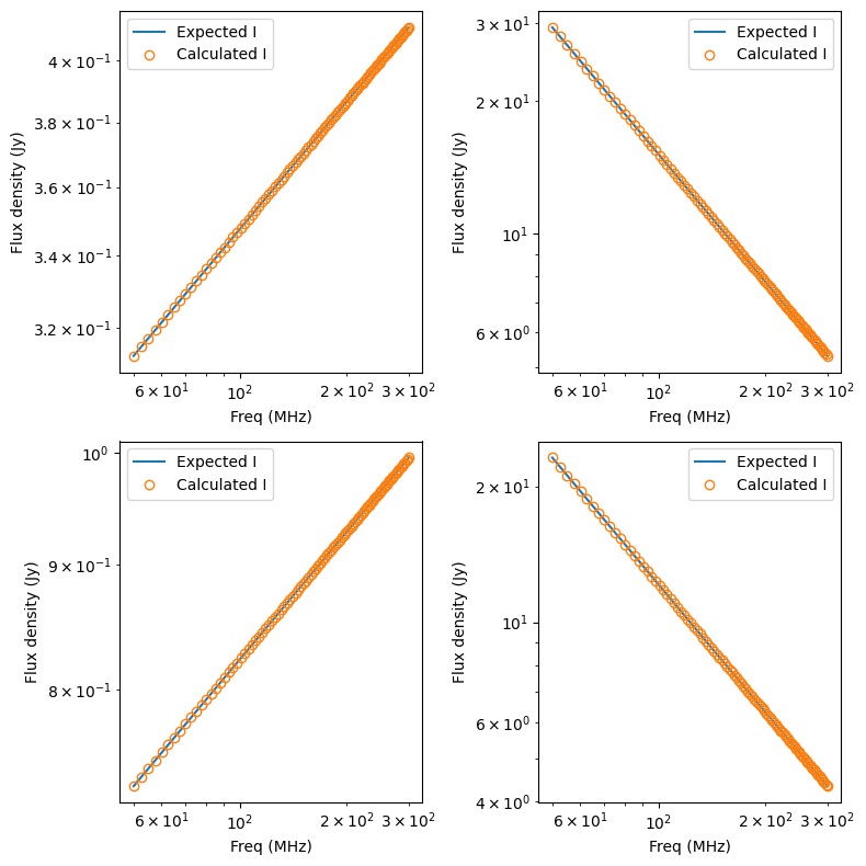
To visualise the Stokes I results, run WODEN/cmake_testing/source_components/test_extrap_stokes.py, which will produce the following plots. The plots only show the Stokes I outputs, but all Stokes values are tested against the C test code.

For the POWER_LAW type components:

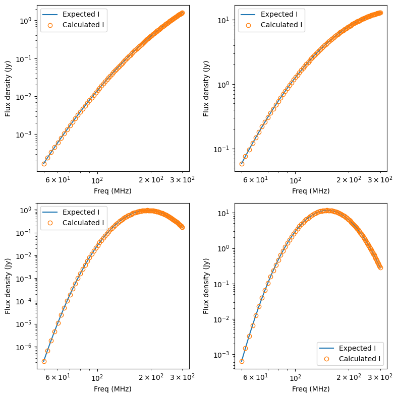
For the CURVED_POWER_LAW type components (where I have set the curve of the peak to be within 100 to 200 MHz so they should all curve in these plots):

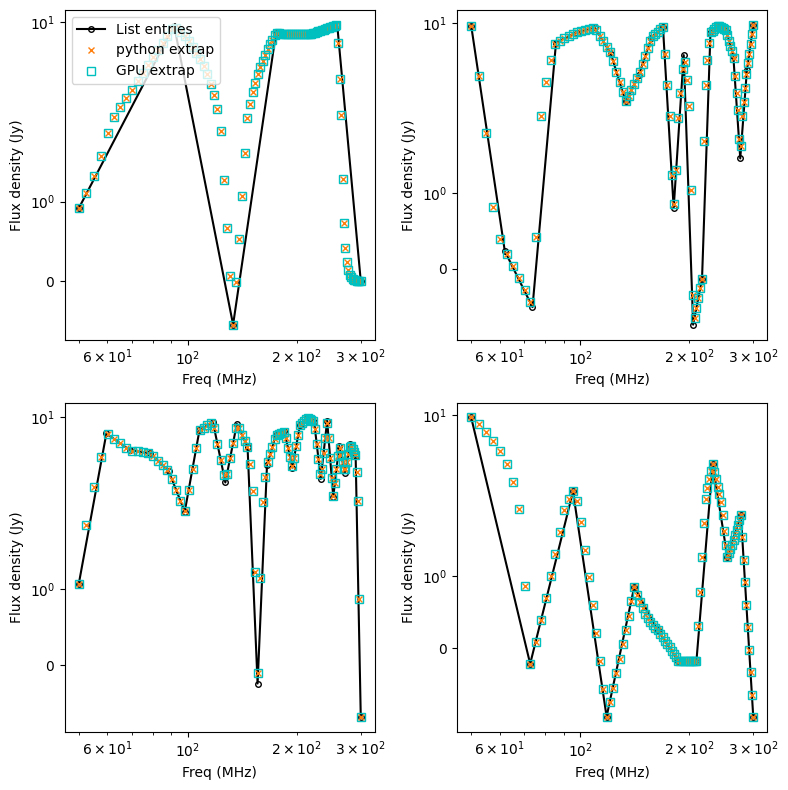
Finally, for the LIST type components. Note here, the black line is the information contained in the sky model, the little orange crosses are a python implementation of the linear interpolation between points to double check everything, and the cyan squares are what is output by the GPU code.

Note

Most SEDs are assumed to be close to a power-law, and so are linear in log space. The linear interpolation is therefore done in log space. However, for some complicated modelling, negative flux values are required. For these values, the interpolation is done in linear space. Hence in the plot below, where the fluxes dip into negative territory, the extrapolated fluxes not longer lie on the straight lines, as these are log-log plots.

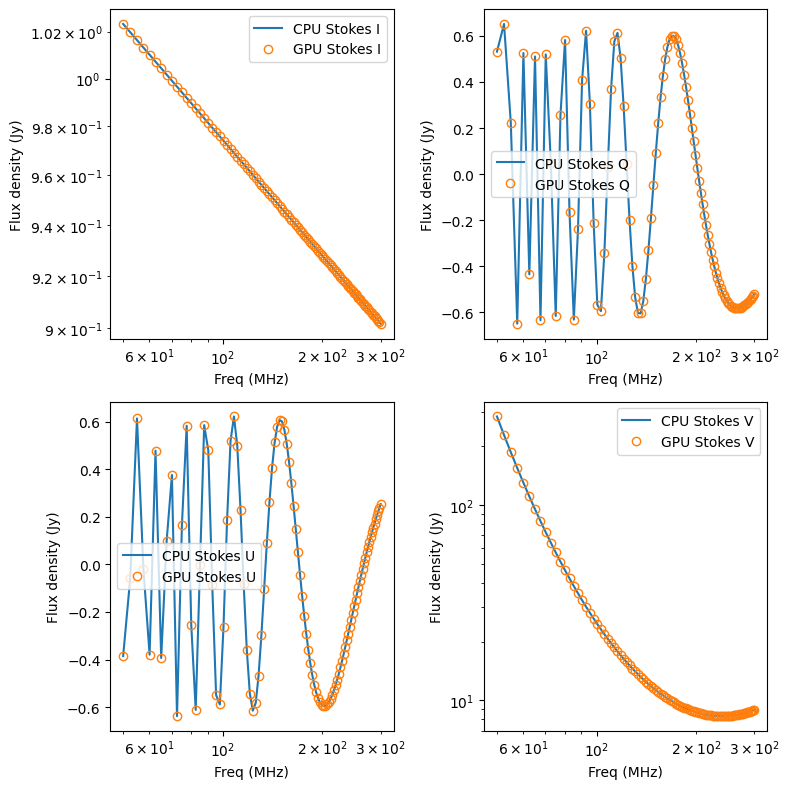
To visualise the full Stokes result for each component, run plot_extrap_stokes.py. An example of a Stokes I power_law, Stokes Q/U polarisation fraction, and Stokes V curved_power_law is:

test_get_beam_gains.c

This calls source_components_gpu.cpp::test_kern_get_beam_gains or source_components_cpu.c::get_beam_gains_cpu. These functions handle grabbing the pre-calculated beam gains for a specific beam model, time, and frequency (assuming the beam gains have already been calculated).

In the test, mock beam gains are stored in primay_beam_J* arrays, including all frequency and time steps, as well as all directions on the sky. This test sets all real entries in the four primay_beam_J* beam gain arrays to the value of their index. In this way, we can easily predict the expected value in the outputs as being the index of the beam gain we wanted to select. I’ve set the imaginary to zero.

This test runs with two time steps, two frequency steps, three baselines, and four beam models. Three different outcomes are expected given the beam model:

• ANALY_DIPOLE, GAUSS_BEAM: The values of the gains are tested to match the expected index. The leakage terms are tested to be zero as the models have no leakage terms

• NO_BEAM: The gain terms are tested to be 1.0, and leakage to be 0.0

• All other beam models: Both the beam gain and leakage terms are tested as these models include leakage terms

test_source_component_common.c

This calls source_components_common.c::source_component_common, which calls source_components::source_component_common. source_component_common is run by all visibility calculation functions (the functions calc_visi_point*, calc_visi_gauss*, calc_visi_shape*). It handles calculating the l,m,n coordinates and beam response for all COMPONENTs in a sky model, regardless of the type of COMPONENT.

Similarly to the tests in test_lmn_coords.c, I setup a slice of 9 RA coordinates, and hold the Dec constant, set the phase centre to RA\(_{\textrm{phase}}\), Dec\(_{\textrm{phase}}\) = \(0^\circ, 0^\circ\). This way I can analytically predict what the l,m,n calculated coordinates should be (which are tested to be within 1e-15 of expected values).

In these tests I run with three time steps, two frequency steps (100 and 200 MHz), and five baselines (the coordinates of which don’t matter, but change the size of the outputs, so good to have a non-one value). I input a set of az,za coords that match the RA,Dec coords for an LST = 0.0. As I have other tests that check the sky moves with time, I just set the sky to be stationary with time here, to keep the test clean.

For each primary beam type, I run the 9 COMPONENTs through the test, and check the calcualted l,m,n are correct, and check that the calculated beam values match a set of expected values, which are stored in test_source_component_common.h. As with previous tests varying the primary beam, I check that leakage terms should be zero when the model doesn’t include them.

Of the nine components tested, 3 are given POWER_LAW, 3 are CURVED_POWER_LAW, and 3 are LIST flux styles. Similarly to test_extrap_stokes.c, each component is given a random set of parameters, and compared to a C version of the functions to extrapolate the Stokes parameters. Again, all components are also give both linear and circular polarisation models.

This test has to create many many input values to run through the function, so is as much of an integration test as a unit test on source_component_common.

test_calc_visi_point*.c

This calls source_components_gpu.cpp::calc_visi_point_or_gauss_gpu of source_components_cpu.c::calc_visi_point_or_gauss_cpu (in this case being used for POINT components). These functions calculate the visibility response for POINT COMPONENTs for a number of sky directions, for all time and frequency steps, and all baselines.

I set up a grid of 25 l,m coords with l,m coords ranging over -0.5, -0.25, 0.0, 0.25, 0.5. I run a simulation with 10 baselines, where I set u,v,w to:

\[\begin{split}u,v = 100(b_{\mathrm{ind}} + 1) \\ w = 10(b_{\mathrm{ind}} + 1)\end{split}\]

where \(b_{\mathrm{ind}}\) is the baseline index, meaning the test covers the baseline range \(100 < u,v <= 1000\) and \(10 < w <= 100\). The test also runs three frequncies, 150, 175, 200 MHz, and two time steps. As I am providing predefined u,v,w, I don’t need to worry about LST effects, but I simulate with two time steps to make sure the resultant visibilities end up in the right order.

Overall, I run three groups of tests here:

• Keeping the beam gains and flux densities constant at 1.0

• Varying the flux densities with frequency and keeping the beam gains constant at 1.0. There are 10 POWER_LAW, 10 CURVED_POWER_LAW, and 5 LIST type components, each with randomly generated values. Equivalent C code is used to calculate the expected fluxes. Some sources are given linear and circular polarisation models; some are not. This tests not only correct polarised flux extrapolation, but also checks those without polarisation information return zeros.

• Varying the beam gains with frequency and keeping the flux densities constant at 1.0. As the beam can vary with time, frequency, and direction on sky, I assign each beam gain a different value. As num_freqs*num_times*num_components = 375, I set the real of all beam gains to \(\frac{1}{375}(B_{\mathrm{ind}} + 1)\), where \(B_{\mathrm{ind}}\) is the beam value index. This way we get a unique value between 0 and 1 for all beam gains, allowing us to test time/frequency is handled correctly by the function under test

Each set of tests is run for all six primary beam types, so a total of 18 tests are called. Each test calls calc_visi_point_or_gauss*, which should calculate the measurement equation for all baselines, time steps, frequency steps, and COMPONENTs. It should also sum over COMPONENTs to get the resultant visibility for each baseline, time, and freq. To test the outputs, I have created equivalent C functions at 64 bit precision in calc_visi_common.c to calculate the measurement equation for the given inputs. Now that we are testing CPU code, it’s a little bit chicken and egg testing the CPU code (which is C code) itself against a stripped down version here in testing. However, if the test code, GPU code, and CPU code all agree, either we’ve made the same bug happen three times in three separate implementations, or we’re correct. Let’s give ourselves the benefit of the doubt.

Note in this tests, I’ve switched to fractional tolerance here as the range of magnitudes covered by these visibilities means a small absolute tolerance will fail a large magnitude visibility when it reports a value that is correct to 1e-11%.

test_calc_visi_gauss*.c

This calls source_components_gpu.cpp::calc_visi_point_or_gauss_gpu of source_components_cpu.c::calc_visi_point_or_gauss_cpu (in this case being used for GAUSSIAN components). These functions calculate the visibility response for GAUSSIAN COMPONENTs for a number of sky directions, for all time and frequency steps, and all baselines.

This runs all tests as described by test_calc_visi_gauss*.c, plus a fourth set of tests that varies the position angle, major, and minor axis of the input GAUSSIAN components, for a total of 24 tests. Again, I have C code to test the CPU/GPU code against. The Gaussian calculations are given a bigger tolerance than the POINT calculations, as the Gaussian envelope that the visibilities are multiplied by adds more precision error.

test_calc_visi_shape*.c

This calls source_components_gpu.cpp::calc_visi_shapelets_gpu or. source_components_cpu.c::calc_visi_shapelets_cpu. These functions calculate the visibility response for SHAPELET COMPONENTs for a number of sky directions, for all time and frequency steps, and all baselines.

This runs all tests as described by test_calc_visi_gauss*.c, plus a fifth set of tests that gives multiple shapelet basis function parameters to the input SHAPELET components, for a total of 30 tests. Again, I have C code to test the CPU/GPU code against.

test_update_sum_visis*.c

This calls source_components_gpu.cpp::kern_update_sum_visis_stokesIQUV or source_components_cpu.c::update_sum_visis_stokesIQUV_cpu. These functions gather pre-calculated primary beam values, unpolarised visibilities, Stokes flux densities, and combines them all into linear polarisation Stokes visibilities. It then sums all COMPONENTs together onto the final set of linear polarisation visibilities.

This code runs three sets of tests, each with three baselines, four time steps, three frequencies, and ten COMPONENTs. For each set of tests, the input arrays that are being tested have their values set to the index of the value, making the summation able to test whether the correct time, frequency, and beam indexes are being summed into the resultant visibilities. The three sets of tests consist of:

• Varying the beam gains, while keeping the flux densities and unpolarised measurement equations constant.

• Varying the flux densities, while keeping the beam gains and unpolarised measurement equations constant.

• Varying the unpolarised measurement equations, while keeping the beam gains and flux densities constant.

Each set of tests is run for all primary beam types, for a total of 18 tests. The different beam models have different expected values depending on whether they include leakage terms or not. Note this test actually doesn’t test with Stokes QUV, it sets QUV to zero. But it’s used in an integration test in test_calculate_visibilities.c with full polarisation.

test_calc_autos*.c

This calls source_components_gpu.cpp::kern_calc_autos or source_components_cpu.c::calc_autos_cpu. This functions gather pre-calculated primary beam values, and Stokes flux densities, and performs a dot-product to calculate the auto-correlations of all antennas, for all time steps.

This test runs by creating full Stokes IQUV model of 4 components, extrapolated to three frequencies and two time steps. Complex beam gains are generated for all directions, times, and frequencies. The auto-correlation calculation is then performed by separate C code, which the outputs of the CPU/GPU code are tested against.

As some primary beam models are real only, and only some have leakage, the function is tested for all beam model types separately, with the expected outcomes calculated accordingly.

test_get_beam_gains_multiants*.c

This works the same as test_get_beam_gains*.c, but we run using a unique primary beam per station (a.k.a tile a.k.a antenna), meaning we input three times the number of gains. Still input each beam gain as it’s index in primay_beam_J. The selected beam gains are now expected to be different for antenna 1 and antenna 2, depending on which visibility they correspond to; they are duly tested to be so. Currently tests using all beams which can produce unique primary beams, which are FEE_BEAM, FEE_BEAM_INTERP, EB_LOFAR, EB_OSKAR (even though the beam values aren’t calculated, check function works as expected with beamtype set).

test_update_sum_visis_multiants*.c

This works similarly to same as test_update_sum_visis*.c, but we run using three unqiue different primary beams, meaning we input three times the number of gains. Still input each beam gain as it’s index in primay_beam_J, which means all three primary beams get different values for every time, freq, direction. Do a bunch of index maths to predict that what value each pair of beam gains should have and check the summed visibilities are correct. Currently tests using all beams which can produce unique primary beams, which are FEE_BEAM, FEE_BEAM_INTERP, EB_LOFAR, EB_OSKAR. (even though the beam values aren’t calculated, check function works as expected with beamtype set).

test_source_component_common_multiants*.c

This works similarly to same as test_source_component_common*.c, but we run using three different primary beams, meaning we calculate three times the number of gains.

We test against stored hyperbeam beam gains for a given set of directions on the sky used in test_source_component_common.c to check it’s calling the primary beam function correctly. However, for each tile/pol, we pass it dipole amplitudes of all of either 0.0, 0.2, 0.4, 0.6, 0.8, 1.0. That way we can just multiply the expected hyperbeam beam gain by the dipole amplitudes to check they’re being implemented and returned correctly. Although this limits the test to only work with FEE_BEAM, FEE_BEAM_INTERP, it tests the order of the outputs, and that most of the machinery to handle multiple primary beams is working correctly.

test_calc_autos_multiants*.c

This calls source_components::test_kern_calc_autos, which in turn calls source_components::kern_calc_autos. This runs the same as test_kern_calc_autos.c, but we run using three different primary beams, meaning we input three times the number of gains. Still input each beam gain as it’s index in primay_beam_J. The selected beam gains are now expected to be different for antenna 1 and antenna 2, depending on which visibility they correspond to; they are duly tested to be so.