Visibility Calculations

Note

Before WODEN version 1.4.0, in the output uvfits files, the first polarisation (usually called XX) was derived from North-South dipoles, as is the labelling convention according to the IAU. However, most uvfits users I’ve met, as well as the data out of the MWA telescope, define XX as East-West. So although the internal labelling and mathematics within the C/CUDA code is to IAU spec, by default, run_woden.py now writes out XX as East-West and YY as North-South. From version 1.4.0, a header value of IAUORDER = F will appear, with F meaning IAU ordering is False, so the polarisations go EW-EW, NS-NS, EW-NS, NS-EW. If IAUORDER = T, the order is NS-NS, EW-EW, NS-EW, EW-NS. If there is no IAUORDER at all, assume IAUORDER = T.

This section assumes a basic understanding on radio interferometry, assuming you know what visibilities and baselines are, and are familiar with the \(u,v,w\) and \(l,m,n\) coordinate systems. I can recommend Thompson, Moran, & Swenson 2017 if you are looking to learn / refresh these concepts. Some of this section is basically a copy/paste from Line et al. 2020.

Note

For WODEN version 2.0.0, the sky model reader has been locked to just reading in Stokes I information, while we wait for the FITS skymodel format. The maths below is still valid, but the sky model reader will only read in Stokes I information. See the Sky model formats for more information.

Measurement Equation and Point Sources

WODEN analytically generates a sky model directly in visibility space via the measurement equation (c.f. Thompson, Moran, & Swenson 2017). Ignoring the effects of instrumental polarisation and the primary beam, this can be expressed as:

\[V_s(u,v,w) = \int \mathcal{S}_s(l,m) \exp[-2\pi i(ul + vm + w(n-1))] \dfrac{dldm}{n},\]

where \(V_s(u,v,w)\) is the measured visibility in some Stokes polarisation \(s\) at baseline coordinates \(u,v,w\), given the sky intensity \(\mathcal{S}\), which is a function of the direction cosines \(l,m\), and \(n=\sqrt{1-l^2-m^2}\). This can be discretised for point sources such that

\[V_s(u_i,v_i,w_i) = \sum_j \mathcal{S}_s(l_j,m_j) \exp[-2\pi i(u_il_j + v_im_j + w_i(n_j-1))],\]

where \(u_i,v_i,w_i\) are the visibility co-ordinates of the \(i^{\mathrm{th}}\) baseline, and \(l_j\), \(m_j\), \(n_j\) is the sky position of the \(j^{\mathrm{th}}\) point source.

Stokes parameters \(\mathcal{S}_I, \mathcal{S}_Q, \mathcal{S}_U, \mathcal{S}_V\) are all extrapolated from an input catalogue, along with the position on the sky. \(u,v,w\) are set by a supplied array layout, phase centre, and location on the Earth.

Note

\(u_i,v_i,w_i\) and \(\mathcal{S}\) are also functions of frequency, so must be calculated for each frequency steps as required.

Apply Linear Stokes Polarisations and the Primary Beam

WODEN simulates dual-linear polarisation antennas, with each antenna/station having it’s own primary beam shape. Typically, these dipoles are aligned north-south and east-west, 0/90 degrees relative to north. I call these “on-cardinal” dipoles. However, some instruments have dipoles that are aligned 45/135 relative to north. I call these “off-cardinal” dipoles. The relative contributions of the Stokes I,Q,U,V parameters to the measured visibilities are different, and therefore are calculated differently internally to WODEN. They are detailed below.

On-cardinal dipoles

I can define the response of a dual polarisation antenna to direction \(l,m\) as

\[\begin{split}\mathbf{J}(l,m) = \begin{bmatrix} g_x(l,m) & D_x(l,m) \\ D_y(l,m) & g_y(l,m) \end{bmatrix},\end{split}\]

where \(g\) are gain terms, \(D\) are leakage terms, and \(x\) refers to a north-south aligned antenna, and \(y\) an east-west aligned antenna. When calculating the cross-correlation responses from antennas 1 and 2 towards direction \(l,m\) to produce linear polarisation visibilities, these gains and leakages interact with the four Stokes polarisations \(I,Q,U,V\) as

\[\begin{split}\begin{bmatrix} V_{12\,XX}(l,m) \\ V_{12\,XY}(l,m) \\ V_{12\,YX}(l,m) \\ V_{12\,YY}(l,m) \end{bmatrix} = \mathbf{J}_1(l,m) \otimes \mathbf{J}_2^*(l,m) \begin{bmatrix} 1 & 1 & 0 & 0 \\ 0 & 0 & 1 & i \\ 0 & 0 & 1 & -i \\ 1 & -1 & 0 & 0 \end{bmatrix} \begin{bmatrix} V_{12\,I}(l,m) \\ V_{12\,Q}(l,m) \\ V_{12\,U}(l,m) \\ V_{12\,V}(l,m) \end{bmatrix}\end{split}\]

where \(*\) denotes a complex conjugate, and \(\otimes\) an outer product. Explicitly, each visibility is

\[\begin{split}\begin{eqnarray*} V_{12\,XX} = (g_{1x}g_{2x}^{\ast} + D_{1x}D_{2x}^{\ast})\mathrm{V}^{I}_{12} + (g_{1x}g_{2x}^{\ast} - D_{1x}D_{2x}^{\ast})\mathrm{V}^{Q}_{12} \\ + (g_{1x}D_{2x}^{\ast} + D_{1x}g_{2x}^{\ast})\mathrm{V}^{U}_{12} + i(g_{1x}D_{2x}^{\ast} - D_{1x}g_{2x}^{\ast})\mathrm{V}^{V}_{12} \end{eqnarray*}\end{split}\]

\[\begin{split}\begin{eqnarray*} V_{12\,XY} = (g_{1x}D_{2y}^{\ast} + D_{1x}g_{2y}^{\ast})\mathrm{V}^{I}_{12} + (g_{1x}D_{2y}^{\ast} - D_{1x}g_{2y}^{\ast})\mathrm{V}^{Q}_{12} \\ + (g_{1x}g_{2y}^{\ast} + D_{1x}D_{2y}^{\ast})\mathrm{V}^{U}_{12} + i(g_{1x}g_{2y}^{\ast} - D_{1x}D_{2y}^{\ast})\mathrm{V}^{V}_{12} \end{eqnarray*}\end{split}\]

\[\begin{split}\begin{eqnarray*} V_{12\,YX} = (D_{1y}g_{2x}^{\ast} + g_{1y}D_{2x}^{\ast})\mathrm{V}^{I}_{12} + (D_{1y}g_{2x}^{\ast} - g_{1y}D_{2x}^{\ast})\mathrm{V}^{Q}_{12} \\ + (D_{1y}D_{2x}^{\ast} + g_{1y}g_{2x}^{\ast})\mathrm{V}^{U}_{12} + i(D_{1y}D_{2x}^{\ast} - g_{1y}g_{2x}^{\ast})\mathrm{V}^{V}_{12} \end{eqnarray*}\end{split}\]

\[\begin{split}\begin{eqnarray*} V_{12\,YY} = (D_{1y}D_{2y}^{\ast} + g_{1y}g_{2y}^{\ast})\mathrm{V}^{I}_{12} + (D_{1y}D_{2y}^{\ast} - g_{1y}g_{2y}^{\ast})\mathrm{V}^{Q}_{12} \\ + (D_{1y}g_{2y}^{\ast} + g_{1y}D_{2y}^{\ast})\mathrm{V}^{U}_{12} + i(D_{1y}g_{2y}^{\ast} - g_{1y}D_{2y}^{\ast})\mathrm{V}^{V}_{12} \end{eqnarray*}\end{split}\]

For each baseline, frequency, and time step, WODEN calculates all four linear polarisations as defined above for all directions \(l_j,m_j\) in the sky model, and then sums over \(j\), to produce four full-sky linear Stokes polarisation visibilities per baseline/frequency/time.

As an aside, if we set the gains to 1 and leakages to zero, we see that

\[\begin{split}\begin{eqnarray*} V_{XX} = \mathrm{V}_{I} + \mathrm{V}_{Q} \\ V_{XY} = \mathrm{V}_{U} + i\mathrm{V}_{V} \\ V_{YX} = \mathrm{V}_{U} - i\mathrm{V}_{V} \\ V_{YY} = \mathrm{V}_{I} - \mathrm{V}_{Q}, \end{eqnarray*}\end{split}\]

meaning to recover the Stokes parameters, imaged visibilities have been beam corrected, we can recover the Stokes parameters as

\[\begin{split}\begin{eqnarray*} \mathrm{V}_{I} = \dfrac{V_{XX} + V_{YY}}{2} \\ \mathrm{V}_{Q} = \dfrac{V_{XX} - V_{YY}}{2} \\ \mathrm{V}_{U} = \dfrac{V_{XY} + V_{YX}}{2} \\ \mathrm{V}_{V} = \dfrac{V_{XY} - V_{YX}}{2i}. \end{eqnarray*}\end{split}\]

Off-cardinal dipoles

Similarly to on-cardinal dipoles, I can define the Jones matrix as

\[\begin{split}\mathbf{J}(l,m) = \begin{bmatrix} g_p(l,m) & D_p(l,m) \\ D_q(l,m) & g_q(l,m) \end{bmatrix},\end{split}\]

where \(g\) are gain terms, \(D\) are leakage terms, \(p\) refers to a 45 degree aligned antenna, and \(q\) a 135 degree aligned antenna. As noted in Table 4.1 of Thompson, Moran, & Swenson 2017, the combinations of Stokes IQUV parameters measured by each instrumental polarisation are different as compared to 0/90 deg dipoles. This means we need a different mixing matrix:

\[\begin{split}\begin{bmatrix} V_{12\,PP}(l,m) \\ V_{12\,PQ}(l,m) \\ V_{12\,QP}(l,m) \\ V_{12\,QQ}(l,m) \end{bmatrix} = \mathbf{J}_1(l,m) \otimes \mathbf{J}_2^*(l,m) \begin{bmatrix} 1 & 0 & 1 & 0 \\ 0 & -1 & 0 & i \\ 0 & -1 & 0 & -i \\ 1 & 0 & -1 & 0 \\ \end{bmatrix} \begin{bmatrix} V_{12\,I}(l,m) \\ V_{12\,Q}(l,m) \\ V_{12\,U}(l,m) \\ V_{12\,V}(l,m) \end{bmatrix},\end{split}\]

where \(*\) denotes a complex conjugate, and \(\otimes\) an outer product. Explicitly, each visibility is

\[\begin{split}\begin{eqnarray*} \mathrm{V}_{12\,PP} = (g_{1p} g_{2p}^* + D_{1p} D_{2p}^*)\mathrm{V}^{I}_{12} - (g_{1p} D_{2p}^* + D_{1p} g_{2p}^*)\mathrm{V}^{Q}_{12} \\+ (g_{1p} g_{2p}^* - D_{1p} D_{2p}^*)\mathrm{U}^{I}_{12} + i(g_{1p} D_{2p}^* - D_{1p} g_{2p}^*)\mathrm{V}^{I}_{12} \end{eqnarray*}\end{split}\]

\[\begin{split}\begin{eqnarray*} \mathrm{V}_{12\,PQ} = (g_{1p} D_{2q}^* + D_{1p} g_{2q}^*)\mathrm{V}^{I}_{12} - (g_{1p} g_{2q}^* + D_{1p} D_{2q}^*)\mathrm{V}^{Q}_{12} \\+ (g_{1p} D_{2q}^* - D_{1p} g_{2q}^*)\mathrm{U}^{I}_{12} + i(g_{1p} g_{2q}^* -D_{1p} D_{2q}^*)\mathrm{V}^{I}_{12} \end{eqnarray*}\end{split}\]

\[\begin{split}\begin{eqnarray*} \mathrm{V}_{12\,QP} = (D_{1q} g_{2p}^* + g_{1q} D_{2p}^*)\mathrm{V}^{I}_{12} - (D_{1q} D_{2p}^* + g_{1q} g_{2p}^*)\mathrm{V}^{Q}_{12} \\+ (D_{1q} g_{2p}^* - g_{1q} D_{2p}^*)\mathrm{U}^{I}_{12} + i(D_{1q} D_{2p}^* -g_{1q} g_{2p}^*)\mathrm{V}^{I}_{12} \end{eqnarray*}\end{split}\]

\[\begin{split}\begin{eqnarray*} \mathrm{V}_{12\,QQ} = (D_{1q} D_{2q}^* + g_{1q} g_{2q}^*)\mathrm{V}^{I}_{12} - (D_{1q} g_{2q}^* + g_{1q} D_{2q}^*)\mathrm{V}^{Q}_{12} \\+ (D_{1q} D_{2q}^* - g_{1q} g_{2q}^*)\mathrm{U}^{I}_{12} + i(D_{1q} g_{2q}^* -g_{1q} D_{2q}^*)\mathrm{V}^{I}_{12} \end{eqnarray*}\end{split}\]

Internally to the WODEN code, everything is labelled as XX, XY, YX, YY, but the above equations are used to calculate the visibilities. Again, if we ignore the beam, we see that

\[\begin{split}\begin{eqnarray*} \mathrm{V}_{QQ} = \mathrm{V}_{I} + \mathrm{V}_{U} \\ \mathrm{V}_{PQ} = -\mathrm{V}_{Q} + i\mathrm{V}_{V} \\ \mathrm{V}_{QP} = -\mathrm{V}_{Q} - i\mathrm{V}_{V} \\ \mathrm{V}_{QQ} = \mathrm{V}_{I} - \mathrm{V}_{U} \end{eqnarray*}\end{split}\]

Rearranging this we see to recover Stokes IQUV visibilities, we obviously need a different set of equations compared to 0/90 deg dipoles. These are

\[\begin{split}\begin{eqnarray*} \mathrm{V}_{I} = \frac{\mathrm{V}_{PP} + \mathrm{V}_{QQ}}{2} \\ \mathrm{V}_{Q} = -\frac{\mathrm{V}_{PQ} + \mathrm{V}_{QP}}{2} \\ \mathrm{V}_{U} = \frac{\mathrm{V}_{PP} - \mathrm{V}_{QQ}}{2} \\ \mathrm{V}_{V} = \frac{\mathrm{V}_{QP} - \mathrm{V}_{PQ}}{2i} \end{eqnarray*}\end{split}\]

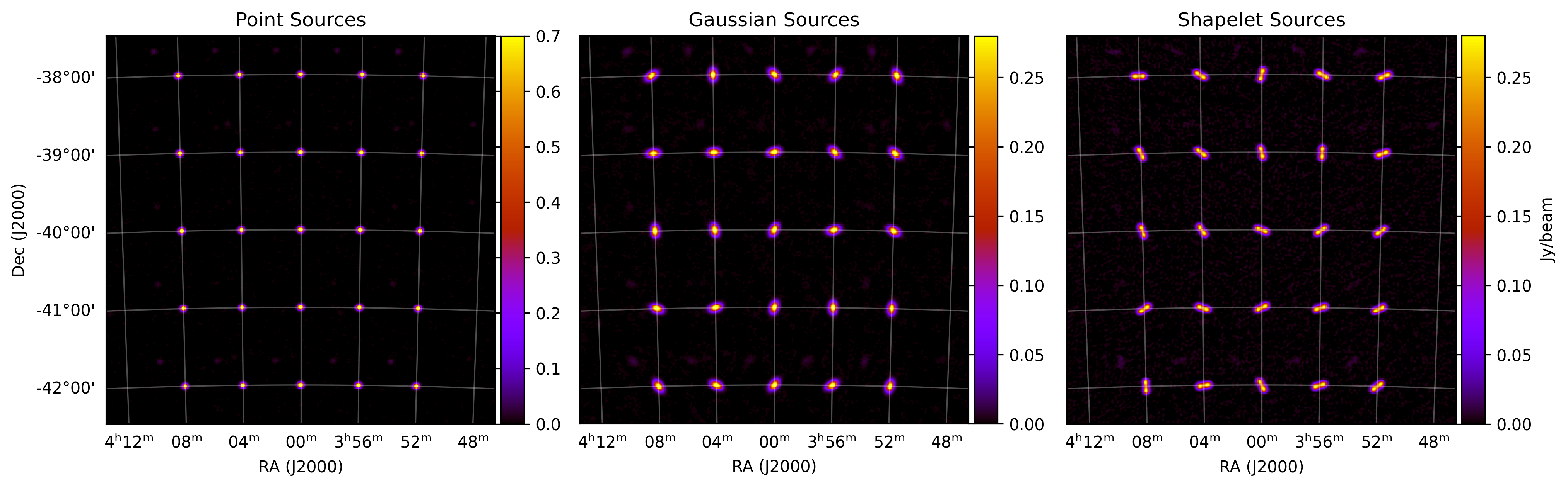
Gaussian and Shapelet sources

You can inject morphology into your sources analytically by tranforming a visibility into a Gaussian or Shapelet source. We utilise the RTS methodology of inserting a visibility “envelope” \(\xi\) into the visibility equation:

\[V(u_i,v_i,w_i) = \sum_j \xi_j(u_i,v_i)\mathcal{S}(l_j,m_j) \exp[-2\pi i(u_il_j + v_im_j + w_i(n_j-1))],\]

For a Gaussian, this envelope looks like

\[\begin{split}\begin{align} &\xi_j = \exp\left( -\dfrac{\pi^2}{4\ln(2)} \left( k_x^2\theta_\mathrm{maj}^2 + k_y^2\theta_\mathrm{min}^2\right) \right); \\ &k_x = \cos(\phi_{\textrm{PA}})v_i + \sin(\phi_{\textrm{PA}})u_i; \\ &k_y = -\sin(\phi_{\textrm{PA}})v_i + \cos(\phi_{\textrm{PA}})u_i; \end{align}\end{split}\]

where \(\theta_\mathrm{maj}\) and \(\theta_\mathrm{min}\) are the major and minor axes and \(\phi_{\textrm{PA}}\) the position angle of an elliptical Gaussian.

For a shapelet model, the envelope looks like:

\[\begin{split}\begin{align} &\xi_j = \sum^{p_k +p_l < p_\mathrm{max}}_{k,l} C_{p_k,p_l} \tilde{B}_{p_k,p_l}(k_x,k_y); \label{eq:shape-env} \\ &k_x = \dfrac{\pi}{\sqrt{2\ln(2)}} \left[\cos(\phi_{PA})v_{i,j} + \sin(\phi_{PA})u_{i,j} \right]; \label{eq:scale-shape-x} \\ &k_y = \dfrac{\pi}{\sqrt{2\ln(2)}} \left[-\sin(\phi_{PA})v_{i,j} + \cos(\phi_{PA})u_{i,j} \right], \label{eq:scale-shape-y} \end{align}\end{split}\]

where \(u_{i,j},v_{i,j}\) are visibility co-ordinates for baseline \(i\), calculated with a phase-centre \(RA_j,\delta_j\), which corresponds to the central position \(x_0,y_0\) used to fit the shapelet model in image-space. The shapelet basis function values \(\tilde{B}_{p_k,p_l}(u,v)\) can be calculated by interpolating from one dimensional look-up tables of \(\tilde{B}(k_x;1)\), and scaling by the appropriate \(\beta\) (c.f. Equation 1 in Line et al. 2020 - see for a introduction and breakdown of shapelets bais functions).

You can see the difference between the three types of sky model component below. You can generate this plot yourself, checkout the section Grid Component Models.