Sky model

Going forward, only the FITS sky model format is being actively developed. This model has full IQUV polarisation options. The hyperdrive yaml format can be still be used for Stokes I only, as well as the deprecated native WODEN format. The FITS format is by far the most efficient in terms of read speed and manipulation however, and so I strongly suggest you suggest you use that format, as well as being able to add QUV information. Below, we’ll define how the spectral information is used by WODEN, and then specify the format of the FITS model.

Spectral models

Stokes I

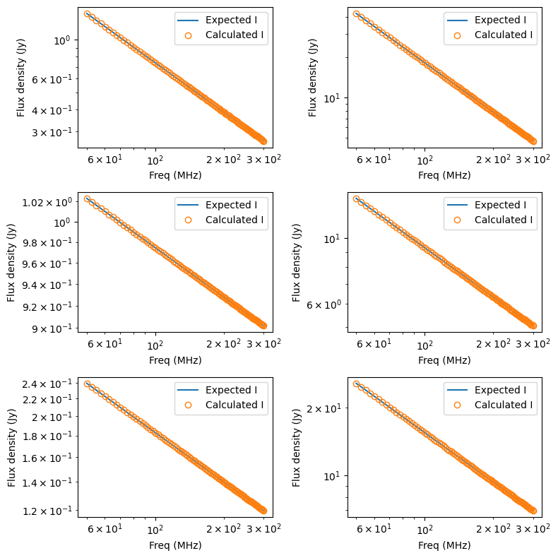
There are three spectral model types for Stokes I: power_law; curved_power_law; list. The power_law model is a simple power law with:

\[S_i = S_0 \left( \frac{\nu_i}{\nu_0} \right)^\alpha\]

where \(S_i\) is the flux density extrapolated to frequency \(\nu_i\), with a reference flux density \(S_0\), reference frequency \(\nu_0\), and spectral index \(\alpha\). An example of these models (these plots are stolen from unit tests of WODEN):

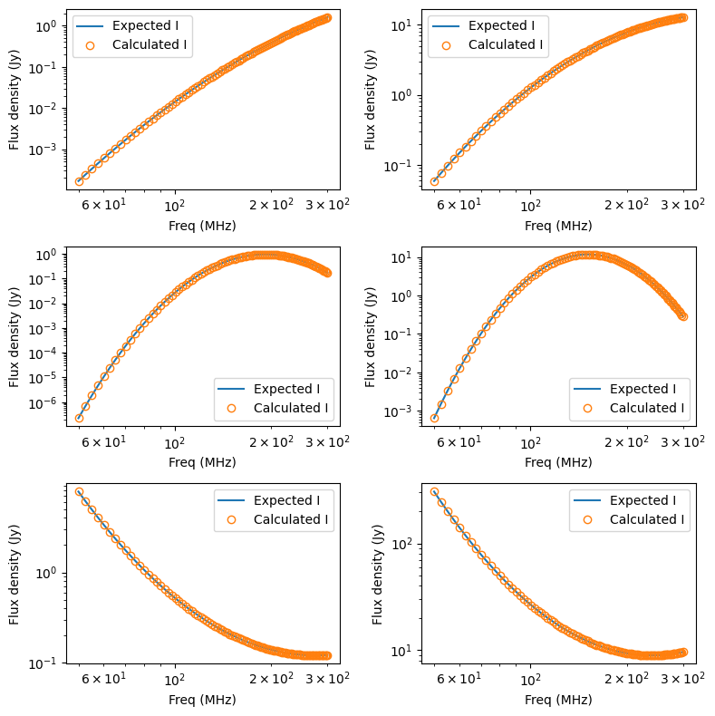
The curved_power_law model is defined in Equation 2 of Callingham et al. 2017, and is implemented in WODEN as:

\[S_i = S_0 \left( \frac{\nu_i}{\nu_0} \right)^\alpha e^{q\ln(\frac{\nu_i}{\nu_0})^2}\]

where \(q\) is a curvature term. This allows for peaked-type SEDs:

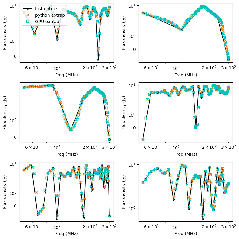
Finally, the list model just takes a list of flux densities, and does a linear interpolation between them. This is useful for simulating things like the 21cm signal which should bounce around with frequency.

Note

Most SEDs are assumed to be close to a power-law, and so are linear in log space. The linear interpolation is therefore done in log space. However, for some complicated modelling, negative flux values are required. For these values, the interpolation is done in linear space. Hence in the plot below, where the fluxes dip into negative territory, the extrapolated fluxes not longer lie on the straight lines, as these are log-log plots. A 21cm list-style SED has been tested to return the expected power spectra, even with this slightly odd log/linear extrapolation combo when bouncing around zero.

Linear polarisation (Stokes Q/U)

The linear polarisation \(P\) can be defined (e.g. Risely et al. 2020) as:

\[P = Q + iU = \mathrm{P}(\lambda) \exp\left( 2i (\chi_0 + \phi_{\textrm{RM}} \lambda^2) \right),\]

where \(Q,U\) are Stokes parameters, \(\mathrm{P}\) is the linear polarisation flux, \(\chi_0\) is the intrinsic polarisation angle, and \(\phi_{\textrm{RM}}\) is the rotation measure.

Using Euler’s formula, this can be used to calculate \(Q,U\) individually:

\[\begin{split}Q = \mathrm{P}(\lambda) \cos(2\chi_0 + 2\phi_{\textrm{RM}} \lambda^2), \\ U = \mathrm{P}(\lambda) \sin(2\chi_0 + 2\phi_{\textrm{RM}} \lambda^2).\end{split}\]

There are five models to calculate the linear polarisation flux \(\mathrm{P}(\lambda)\) in WODEN: power_law; curved_power_law; polarisation fraction; list; p-list. The first two models work exactly the same as the Stokes I models, but with their own reference fluxes and spectral indices. The polarisation fraction model is a simple fraction of the Stokes I flux density, and is defined as:

\[\mathrm{P}(\lambda) = \Pi I(\lambda) ,\]

where \(\Pi\) is the polarisation fraction, and \(I(\lambda)\) is the Stokes I flux density. Note that \(\Pi\) can be negative, and greater than one.

The list model is the same as the Stokes I list model, but the user enters two separate lists for Stokes \(Q\) and \(U\) as a function of frequency. This means \(Q\)/\(U\) are extrapolated independently of one another, and not related via \(\phi_{\textrm{RM}}\). With the p-list model the user enters a list of \(\mathrm{P}(\lambda)\) fluxes, which is used in conjunction with the rotation measure to calculate \(Q\) and \(U\). See below for exactly how to input these lists using the FITS format.

Circular polarisation (Stokes V)

Similarly to linear polarisation, circular polarisation can be calculated via three different models: power_law; curved_power_law; polarisation fraction; list. Again, both power_law and curved_power_law mean Stokes V will be modelled separately from Stokes I. polarisation fraction is again a fraction of the Stokes I flux density. Finally list is a list of flux densities as a function of frequency, and WODEN will interpolate between these values.

Example of a full Stokes SED

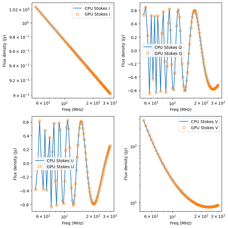
An example of these models for a single component (again, plots made using unit tests out of WODEN) is below. Here, Stokes I is a power_law, Stokes Q/U are a polarisation fraction, and Stokes V is a curved_power_law:

Sky model formats

In WODEN nomenclature (which was inherited from the oracle RTS), each astrophysical object is called a SOURCE. Each SOURCE can have multiple components, which are called COMPONENTs. Each COMPONENT can be a point source, Gaussian, or shapelet.

FITS sky model format

This sky model follows (and expands upon) the format of the LoBES catalogue Lynch et al. 2021 and is the preferred format as it’s the fastest and easiest to lazy load. There are three COMPONENT types: point source; Gaussian; shapelets. These are all the model types as defined in Line et al. 2020 (including the mathematics of how each model is simulated). You can create any number of SOURCEs, each with any number of COMPONENTs, by using the UNQ_SOURCE_ID and NAME columns as detailed below. The sky model is a FITS file with at least one HDU (must appear first, and best to be given name MAIN) with the following columns. Unless otherwise stated, all columns are optional (e.g. if you don’t want to include polarisation information, you can leave out the polarisation columns):

MAIN HDU

Column Name	Unit	Description
UNQ_SOURCE_ID		(Required) Unique source ID. This is used to group COMPONENTs into SOURCEs. If you want to have multiple components in a single source, they must have the same UNQ_SOURCE_ID.
NAME		(Required) This is a COMPONENT name, and should read as UNQ_SOURCE_ID_C`number` where `number` is a COMPONENT number. For example, if you have a SOURCE with UNQ_SOURCE_ID = FornaxA, and you have two components, you should have two rows with NAME = FornaxA_C000 and FornaxA_C001.
RA	deg	(Required) Right Ascension (J2000)
DEC	deg	(Required) Declination (J2000)
COMP_TYPE		(Required) Specifies if the component is a point source, Gaussian, or shapelet. Entered as either P, G, or S.
MAJOR_DC	deg	Major axis of Gaussian or shapelet model
MINOR_DC	deg	Minor axis of Gaussian or shapelet model
PA_DC	deg	Position angle of Gaussian or shapelet model
MOD_TYPE		(Required) The Stokes I flux model of this component. Can be either pl (power-law), cpl (curved power-law), or nan (list of flux densities).
NORM_COMP_PL	Jy	The Stokes I reference flux for a power-law pl component model, must be at the reference frequency 200MHz.
ALPHA_PL		The sStokes I pectral index for a power-law pl component model
NORM_COMP_CPL	Jy	The Stokes I reference flux for a curved power-law cpl component model, must be at the reference frequency 200MHz.
ALPHA_CPL		The Stokes I spectral index for a curved power-law cpl component model, must be at the reference frequency 200MHz.
CURVE_CPL		The Stokes I curvature q for a curved power-law cpl component model
INT_FLX*frequency*	Jy	A reference Stokes I flux density, where frequency is the frequency in MHz. For a list type flux model, you can include as many INT_FLX*frequency* columns as necessary. For example, if you have three reference fluxes at 100, 150, and 200 MHz, you should have three columns INT_FLX100, INT_FLX150, and INT_FLX200.
V_MOD_TYPE		The Stokes V flux model of this component. Can be either pl (power-law), cpl (curved power-law), or pf (polarisation fraction).
V_POL_FRAC		The Stokes V polarisation fraction; can be negative, and greater than one.
V_NORM_COMP_PL	Jy	The Stokes V reference flux for a power-law pl component model, must be at the reference frequency 200MHz.
V_ALPHA_PL		The Stokes V pectral index for a power-law pl component model
V_NORM_COMP_CPL	Jy	The Stokes V reference flux for a curved power-law cpl component model, must be at the reference frequency 200MHz.
V_ALPHA_CPL		The Stokes V spectral index for a curved power-law cpl component model, must be at the reference frequency 200MHz.
V_CURVE_CPL		The Stokes V curvature q for a curved power-law cpl component model
LIN_MOD_TYPE		The linear polarisation flux model of this component. Can be either pl (power-law), cpl (curved power-law), or pf (polarisation fraction).
RM	rad/m^2	The rotation measure of the linear polarisation
INTR_POL_ANGLE	rad	The intrinsic polarisation angle of the linear polarisation; if this column is missing, assume 0 degrees.
LIN_POL_FRAC		The linear polarisation fraction; can be negative, and greater than one.
LIN_NORM_COMP_PL	Jy	The Linear Polarisation flux reference flux for a power-law pl component model, must be at the reference frequency 200MHz.
LIN_ALPHA_PL		The Linear Polarisation flux pectral index for a power-law pl component model
LIN_NORM_COMP_CPL	Jy	The Linear Polarisation flux reference flux for a curved power-law cpl component model, must be at the reference frequency 200MHz.
LIN_ALPHA_CPL		The Linear Polarisation flux spectral index for a curved power-law cpl component model, must be at the reference frequency 200MHz.
LIN_CURVE_CPL		The Linear Polarisation flux curvature q for a curved power-law cpl component model

If you want to include SHAPELETS, you must include a second HDU that details the shapelet basis functions for each component, using the following columns. If the table does not appear directly after the MAIN table, it must be given the name SHAPELET:

SHAPELET HDU

Column Name	Description
NAME	The COMPONENT name exactly as appears in the first HDU NAME column. You can have multiple rows for each COMPONENT, each with a unique combination of N1, N2, and COEFF, to include as many shapelet basis functions as necessary. WODEN will cross-reference the two HDUs to use these basis functions in conjunction with the position and flux model in the first HDU.
N1	The first shapelet order
N2	The second shapelet order
COEFF	The coefficient to multiply this basis function by

The SHAPELET HDU is optional, and if it is not present, WODEN will assume all components are either point sources or Gaussians.

Polarisation list-style flux tables

If you want to include polarised list-style information, besides setting nan in the V_MOD_TYPE and/or nan / p_nan in the LIN_MOD_TYPE columns, you must include extra HDUs that contain the listed fluxes. See WODEN/examples/polarisation/polarisation_examples.ipynb for example Python code to create these tables.

To include a list of Stokes V fluxes, you must include an HDU with the name V_LIST_FLUXES (it MUST be named). This HDU must have the following columns:

V_LIST_FLUXES HDU

Column Name	Unit	Description
NAME		The COMPONENT name exactly as appears in the MAIN HDU NAME column. WODEN will cross-reference the two HDUs to link the RA/DEC / Stokes I information for the COMPONENT.
V_INT_FLX*frequency*	Jy	A reference Stokes V flux density, where frequency is the frequency in MHz. For a list type flux model, you can include as many V_INT_FLX*frequency* columns as necessary. For example, if you have three reference fluxes at 100, 150, and 200 MHz, you should have three columns V_INT_FLX100, V_INT_FLX150, and V_INT_FLX200.

If you set p_nan in the LIN_MOD_TYPE columns, it means you want to include a list of polarised flux densities (\(P(\nu)\)). These are used in conjunction with the RM and INTR_POL_ANGLE columns in the MAIN HDU to calculate Stokes Q/U. You must include an HDU with the name P_LIST_FLUXES (it MUST be named). This HDU must have the following columns:

P_LIST_FLUXES HDU

Column Name	Unit	Description
NAME		The COMPONENT name exactly as appears in the MAIN HDU NAME column. WODEN will cross-reference the two HDUs to link the RA/DEC / Stokes I information for the COMPONENT.
P_INT_FLX*frequency*	Jy	A reference linear polarised flux density, where frequency is the frequency in MHz. For a list type flux model, you can include as many P_INT_FLX*frequency* columns as necessary. For example, if you have three reference fluxes at 100, 150, and 200 MHz, you should have three columns P_INT_FLX100, P_INT_FLX150, and P_INT_FLX200.

If you set nan in the LIN_MOD_TYPE columns, it means you want to include separate lists for Stokes Q and U. These lists will be used to extrapolate the Q and U fluxes separately. You must include two extra HDUs with the names Q_LIST_FLUXES and U_LIST_FLUXES (they MUST be named). Both HDUs must include the same number of COMPONENTs, as WODEN will try to extrapolate the Q/U fluxes for every nan entry in the LIN_MOD_TYPE column in the MAIN HDU. The HDUs must have the following columns:

Q_LIST_FLUXES HDU

Column Name	Unit	Description
NAME		The COMPONENT name exactly as appears in the MAIN HDU NAME column. WODEN will cross-reference the two HDUs to link the RA/DEC / Stokes I information for the COMPONENT.
Q_INT_FLX*frequency*	Jy	A reference Stokes Q flux density, where frequency is the frequency in MHz. For a list type flux model, you can include as many Q_INT_FLX*frequency* columns as necessary. For example, if you have three reference fluxes at 100, 150, and 200 MHz, you should have three columns Q_INT_FLX100, Q_INT_FLX150, and Q_INT_FLX200.

U_LIST_FLUXES HDU

Column Name	Unit	Description
NAME		The COMPONENT name exactly as appears in the MAIN HDU NAME column. WODEN will cross-reference the two HDUs to link the RA/DEC / Stokes I information for the COMPONENT.
U_INT_FLX*frequency*	Jy	A reference Stokes P flux density, where frequency is the frequency in MHz. For a list type flux model, you can include as many U_INT_FLX*frequency* columns as necessary. For example, if you have three reference fluxes at 100, 150, and 200 MHz, you should have three columns U_INT_FLX100, U_INT_FLX150, and U_INT_FLX200.