LOFAR LoTSS DR2 cutout matching

In this example, we’ll take a chunk of the LoTSS_DR2_v110.gaus.fits LOFAR source catalogue, convert it to a WODEN sky model, run it through a WODEN simulation, and try and match a postage stampl cutout from the actual LoTSS survey.

First up, what let’s look at what we’re trying to emulate. I went to the LoTSS DR2 cutout service and grabbed the nearest cut out to RA, Dec = 180.0, 50.0. That retuned the P18Hetdex03 field, which looks like this:

from astropy.io import fits
from astropy.wcs import WCS
import numpy as np 

with fits.open('P18Hetdex03_mosaic-blanked.fits') as hdu:
    wcs = WCS(hdu[0].header).celestial
    pix_res = np.abs(hdu[0].header['CDELT1'])
    cent_x = hdu[0].header['CRPIX1']
    cent_y = hdu[0].header['CRPIX2']
    
    cent_ra = hdu[0].header['CRVAL1']
    cent_dec = hdu[0].header['CRVAL2']
    
    cat_freq = hdu[0].header['RESTFRQ']
    
    data = np.squeeze(hdu[0].data)

import matplotlib.pyplot as plt

fig, axs = plt.subplots(1, 1, subplot_kw={'projection': wcs}, figsize=(12, 10))
im = axs.imshow(data, origin='lower', cmap='Blues', vmin=0, vmax=1e-3)

half_width=2048

axs.set_xlim(cent_x - half_width, cent_x + half_width)
axs.set_ylim(cent_y - half_width, cent_y + half_width)


axs.set_xlabel('RA')
axs.set_ylabel('Dec')

plt.colorbar(im, ax=axs, label='Flux (Jy/beam)')
plt.show()

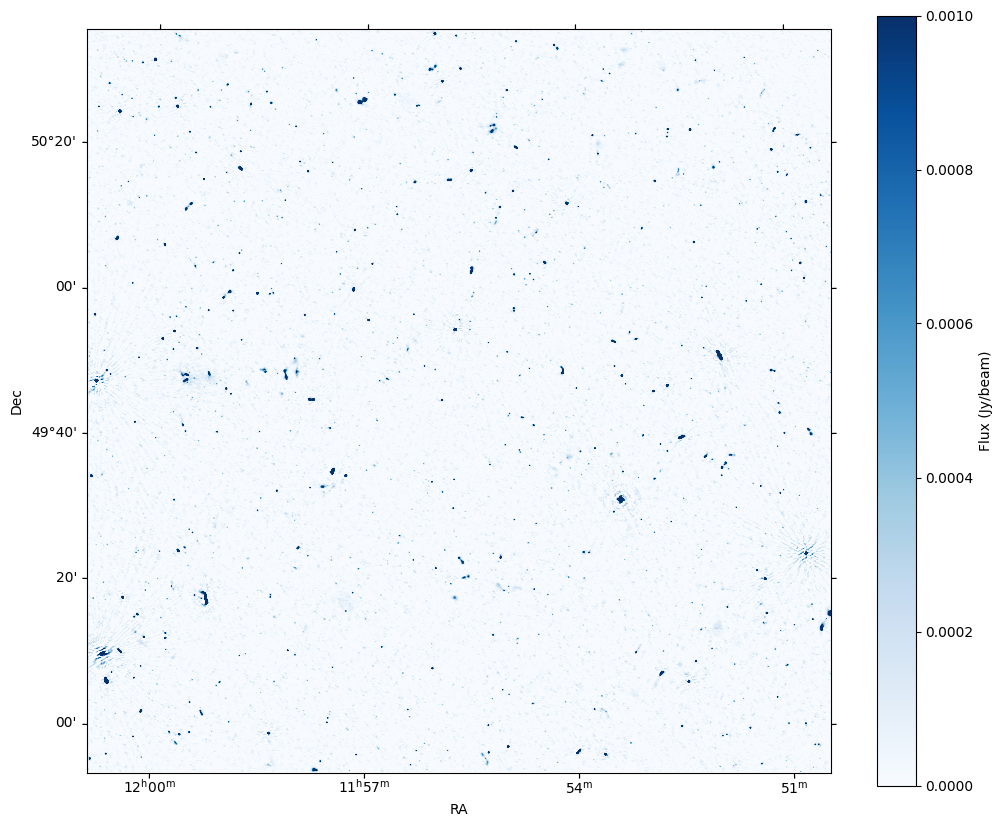
That’s a spicy meatball! Super high res and deep image. Checking the LoTSS data products page I can find Non-redundant Gaussian catalogue v1.1. Clicking that downloads the LoTSS_DR2_v110.gaus.fits file. Hopefully as this is a Gaussian catalogue, it should give us a realistic looking sky model. First up, let’s load the catalogue.

from astropy.table import Table
from astropy.coordinates import SkyCoord

table_lotss = Table.read('LoTSS_DR2_v110.gaus.fits')
unq_source_ids = np.array(table_lotss['Source_Name'], dtype='U32')
##order everything by source name to make adding converting into a WODEN
##style table easier
ordering = np.argsort(unq_source_ids)
unq_source_ids = unq_source_ids[ordering]
ras = table_lotss['RA'][ordering]
decs = table_lotss['DEC'][ordering]
fluxes = table_lotss['Total_flux'][ordering]/1000.0
majors = table_lotss['DC_Maj'][ordering]/3600.0
minors = table_lotss['DC_Min'][ordering]/3600.0
pas = table_lotss['PA'][ordering]


##Make some astropy skycoords
coords = SkyCoord(ras, decs, unit='deg')
##Make a skycoord for the image centre
image_centre = SkyCoord(cent_ra, cent_dec, unit='deg')
##Find separation of all catalogue sources from image centre
separations = image_centre.separation(coords).degree

Next, we’ll trim to catalogue down to sources that fit within a degree from the centre of our cutout image. Plot it over the cutout image to sanity check everything.

subset = np.where(separations < 1.0)


ra_subset = ras[subset]
dec_subset = decs[subset]

x_sub, y_sub = wcs.all_world2pix(ra_subset, dec_subset, 0)


fig, axs = plt.subplots(1, 1, subplot_kw={'projection': wcs}, figsize=(12, 10))
im = axs.imshow(data, origin='lower', cmap='Blues', vmin=0, vmax=1e-3)

axs.scatter(x_sub, y_sub, marker='.', s=2, edgecolor='C1', alpha=1.0)

half_width=2048

axs.set_xlim(cent_x - half_width, cent_x + half_width)
axs.set_ylim(cent_y - half_width, cent_y + half_width)


axs.set_xlabel('RA')
axs.set_ylabel('Dec')

plt.colorbar(im, ax=axs, label='Flux (Jy/beam)')
plt.show()

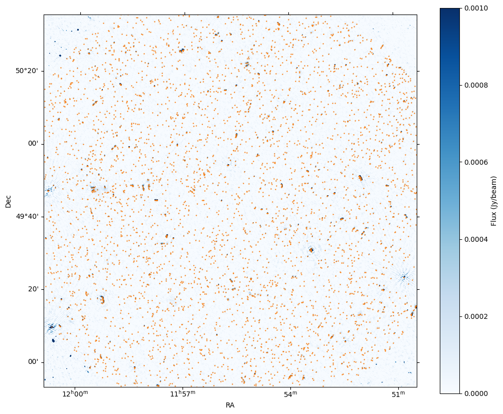
We’ve defo go the correct coverage! Weirdly, all the sources seem slightly offset from the cutout image. Maybe the catalogue has been ionospherically corrected and the image hasn’t? Anyways, should still be good enough to run through WODEN. Let’s convert it to something that WODEN can understand.

##First up, only use the subset we've just defined
num_comps = len(subset[0])

unq_source_ids_use = unq_source_ids[subset]
ras_use = ras[subset]
decs_use = decs[subset]
fluxes_use = fluxes[subset]
majors_use = majors[subset]
minors_use = minors[subset]
pas_use = pas[subset]
##Catalogue doesn't see to come with spectral index so just set to -0.8
alphas = np.full(num_comps, -0.8)

print('Number of components:', num_comps)

Number of components: 4995

Next, get the naming convention that the WODEN catalogue needs (based on the LoBES survey, also used by hyperdrive). It needs to have a column called UNQ_SOURCE_ID, which is the name of the parent source for any catalogue entry. It also needs a NAME column, which is the name of the parent source plus f"_C{comp_ind}" where comp_ind is the component index within that source. WODEN uses this to group components from the same source together, useful if you want to crop below the horizon by source.

Anyways, we’ve loaded the Source_Name column from the LoTSS catalogue as unq_source_ids. So we can use this to form the NAME column.

##Grabs all unique names, the indexes of the first occurance, and how many times
##that name appears
unq_names, unq_indexes, unq_counts = np.unique(unq_source_ids_use, return_index=True, return_counts=True)

names = np.empty(num_comps, dtype='U32')
for unq_name, unq_index, unq_count in zip(unq_names, unq_indexes, unq_counts):
    ##If there is more than one component with the same name, iterate
    ##over them            
    if unq_count > 1:
        for comp_id in range(unq_count):
            names[unq_index + comp_id] = f"{unq_name}_C{comp_id:03d}"
    ##Otherwise just set the name to the original name + C000
    else:
        names[unq_index] = f"{unq_name}_C000"
        

Beyond that, fluxes are all reported at 200 MHz, so we need to scale from the native 144 MHz. Again, just assume we have spectral index of -0.8 everywhere for this.

extrap_freq = 200e+6
alpha = -0.8
fluxes_extrap = fluxes_use*(extrap_freq/cat_freq)**alpha

One other WODEN thing we need is the COMP_TYPE column, that tells us whether it’s a Gaussian or a Point source. We’ll set anything with a Major axis of 0 as a point source.

comp_types = np.empty(num_comps, dtype='U3')
comp_types[majors_use == 0.0] = 'P'
comp_types[majors_use != 0.0] = 'G'

Now we just reassemble the other columns with new names and write out the catalogue.

from astropy.table import Column

unq_source_id_col = Column(unq_source_ids_use, name='UNQ_SOURCE_ID')
names_col = Column(names, name='NAME')

ras_col = Column(ras_use, name='RA', unit='deg')
decs_col = Column(decs_use, name='DEC', unit='deg')
fluxes_col = Column(fluxes_extrap, name='NORM_COMP_PL', unit='Jy')
si_col = Column(alphas, name='ALPHA_PL', unit='Jy')
majors_col = Column(majors_use, name='MAJOR_DC', unit='deg')
minors_col = Column(majors_use, name='MINOR_DC', unit='deg')
pas_col = Column(pas_use, name='PA_DC', unit='deg')
comp_types_col = Column(comp_types, name='COMP_TYPE')
##We're inputting everything as a power law
mod_types_col = Column(np.full(num_comps, 'pl'), name='MOD_TYPE')

cols = [unq_source_id_col, names_col,
        ras_col, decs_col, comp_types_col, mod_types_col,
        fluxes_col, si_col,
        majors_col, minors_col, pas_col]

new_table = Table(cols)
new_table.write('srclist_LoTSS_DR2_v110.gaus_P18Hetdex03.fits', overwrite=True)

OK! Let’s try and do a simulation to match this. Would be nice to find a date that sticks the LST of the observation as close to overhead as possible. Everyone loves a zenith pointing. I’m not doing this intelligently here. I just fiddle the time until it was pretty close.

from astropy.time import Time
from astropy.coordinates import EarthLocation
import astropy.units as u


lofar_lat = 52.905329712
lofar_long = 6.867996528

##pick a time/date that sticks our phase centre overhead
##Picking a random time on the day I'm writing this
date = "2024-11-12T08:00:26"

lofar_location = EarthLocation(lat=lofar_lat*u.deg, 
                               lon=lofar_long*u.deg)

observing_time = Time(date, scale='utc', location=lofar_location)

##Grab the LST
LST = observing_time.sidereal_time('mean')
LST_deg = LST.value*15
print(f"LST: {LST_deg} deg, Image centre: {cent_ra} deg")

LST: 178.92258388645152 deg, Image centre: 178.922 deg

OK, so the LoTSS survey was done with high-band antennas, so we need a measurement to match that. I’m using LOFAR_HBA_MOCK.ms, which is an MS used in EveryBeam test suite. We want a nice clean image, so we’ll try and do some rotation synthesis. WODEN is currently defaulted to using locking the EveryBeam primary beam to the phase centre. So we’ll do a 10 hour observation. To keep the simulation managable on my desktop, I’ll sample every 15 minutes. I’ll do 40 frequency channels, spread over a 20MHz bandwidth.

Note I add --max_sky_directions=10 to limit the number of sky directions, and therefore components, per sky model chunk. This is because we have 40 time steps, 40 frequencies, so for 10 directions, that’s 40x40x10 = 16000 beam calculations per station. This keeps things down to a managable size before handing off the beam values to the GPU. This is something that needs to be optimised and better automated by the code in the future.

##You can run all this normally on the command line via run_woden.py
##Here, I'm going to load main from run_woden.py and run it directly,
##supply a list of arguments as if they were command line arguments
import sys
sys.path.append('../../scripts')
from run_woden import main as run_woden
import numpy as np

ms_path='../../test_installation/everybeam/LOFAR_HBA_MOCK.ms'
uvfits_name='woden_P18Hetdex03'
cat_name='srclist_LoTSS_DR2_v110.gaus_P18Hetdex03.fits'
primary_beam='everybeam_LOFAR'

mid_freq = 144e+6
bandwidth = 20e+6
num_freqs = 40
freqs = np.linspace(mid_freq - bandwidth/2, mid_freq + bandwidth/2, num_freqs)

freq_reso = freqs[1] - freqs[0]
num_freq_chans = len(freqs)
low_freq = freqs[0]

##Do a tracked observation for +/- 5 hours
##Start 5 hours before our field centre is overhead
date = "2024-11-12T03:00:26"

##Every 15 mins for 40 time steps is 10 hours
time_res = 900.0
num_times = 40

args = []

##The command to run WODEN
args.append(f'--ra0={cent_ra}')
args.append(f'--dec0={cent_dec}')
args.append(f'--latitude={lofar_lat}')
args.append(f'--longitude={lofar_long}')
args.append(f'--date={date}')
args.append(f'--output_uvfits_prepend={uvfits_name}')
args.append(f'--cat_filename={cat_name}')
args.append(f'--primary_beam={primary_beam}')
args.append(f'--lowest_channel_freq={low_freq}')
args.append(f'--freq_res={freq_reso}')
args.append(f'--num_freq_channels={num_freq_chans}')
args.append(f'--band_nums=1')
args.append(f'--time_res={time_res}')
args.append(f'--num_time_steps={num_times}')
args.append(f'--IAU_order')
args.append(f'--max_sky_directions=50')
args.append('--num_threads=8')
args.append(f'--beam_ms_path={ms_path}')
args.append(f'--max_sky_directions=10')

print(args)
# run_woden(args)

['--ra0=178.922', '--dec0=49.748', '--latitude=52.905329712', '--longitude=6.867996528', '--date=2024-11-12T03:00:26', '--output_uvfits_prepend=woden_P18Hetdex03', '--cat_filename=srclist_LoTSS_DR2_v110.gaus_P18Hetdex03.fits', '--primary_beam=everybeam_LOFAR', '--lowest_channel_freq=134000000.0', '--freq_res=512820.51282051206', '--num_freq_channels=40', '--band_nums=1', '--time_res=900.0', '--num_time_steps=40', '--IAU_order', '--max_sky_directions=50', '--num_threads=8', '--beam_ms_path=../../test_installation/everybeam/LOFAR_HBA_MOCK.ms', '--max_sky_directions=10']

Note that I ended up running the simulation on the command line, via the print statement. The output is super long so didn’t want to make the notebook forever long. It took just under an hour on my desktop.

OK, let’s see what we get! First up, what uv coverage do we get?

from astropy.constants import c
c = c.to('m/s').value

with fits.open('woden_P18Hetdex03_band01.uvfits') as hdu:
    uu = (hdu[0].data['UU']*c)/1e+3
    vv = (hdu[0].data['VV']*c)/1e+3
    
fig, axs = plt.subplots(1, 1, figsize=(8, 8))
axs.plot(uu, vv, 'k.', ms=1)
axs.plot(-uu, -vv, 'k.', ms=1)
axs.set_xlabel('U (km)')
axs.set_ylabel('V (km)')

plt.show()

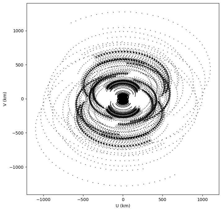
Thems some long baselines. Convert the UVFITS to an MS. Below is the function that’s in woden_uv2ms.py. Just copied it here to show what’s going on.

from pyuvdata import UVData
from subprocess import call
import os

def make_ms(uvfits_file, no_delete=False):
    """Takes a path to a uvfits file, checks it exists, and converts it to
    a measurement set of the same name at the same location"""

    ##If file exists, attempt to tranform it
    if os.path.isfile(uvfits_file):
        ##Get rid of '.uvfits' off the end of the file
        name = uvfits_file[:-7]
        ##Delete old measurement set if requested
        if no_delete:
            pass
        else:
            call("rm -r %s.ms" %name,shell=True)

        UV = UVData()
        UV.read(uvfits_file)
        
        UV.write_ms("{:s}.ms".format(name))
        
    else:
        ##print warning that uvfits file doesn't exist
        print("Could not find the uvfits specified by the path: "
              "\t{:s}. Skipping this tranformation".format(uvfits_file))
        

make_ms('woden_P18Hetdex03_band01.uvfits')

The telescope frame is set to '????', which generally indicates ignorance. Defaulting the frame to 'itrs', but this may lead to other warnings or errors.
The uvw_array does not match the expected values given the antenna positions. The largest discrepancy is 84.13106539141154 meters. This is a fairly common situation but might indicate an error in the antenna positions, the uvws or the phasing.
The uvw_array does not match the expected values given the antenna positions. The largest discrepancy is 84.13106539141154 meters. This is a fairly common situation but might indicate an error in the antenna positions, the uvws or the phasing.
Writing in the MS file that the units of the data are uncalib, although some CASA process will ignore this and assume the units are all in Jy (or may not know how to handle data in these units).

cmd = 'wsclean -name woden_P18Hetdex03 -niter 20000 '
cmd += '   -size 4096 4096 -scale 1.5asec '
cmd += '   -weight briggs 0 '
cmd += '   -auto-threshold 0.5 -auto-mask 3 -pol I -multiscale '
cmd += '   -j 12 -mgain 0.85 -no-update-model-required '
cmd += '   -beam-size 6 '
cmd += '   -abs-mem 25 '
cmd += '   woden_P18Hetdex03_band01.ms'

##My local WSClean installation is borked, so I have to print the command and run it manually
print(cmd)
# call(cmd, shell=True)

wsclean -name woden_P18Hetdex03 -niter 20000    -size 4096 4096 -scale 1.5asec    -weight briggs 0    -auto-threshold 0.5 -auto-mask 3 -pol I -multiscale    -j 12 -mgain 0.85 -no-update-model-required    -beam-size 6    -abs-mem 25    woden_P18Hetdex03_band01.ms

I’m sure this isn’t an optimal way to do the CLEANing, and I might be able to go deeper, but this is good enough for a comparison. Let’s see what we get!

fig = plt.figure(figsize=(9, 11))

ax1 = fig.add_subplot(211, projection=wcs)
ax1.imshow(data, origin='lower', cmap='Blues', vmin=0, vmax=1e-3)

half_width=2048

ax1.set_xlim(cent_x - half_width, cent_x + half_width)
ax1.set_ylim(cent_y - half_width, cent_y + half_width)

vmax = 5e-3

im = ax1.imshow(data, origin='lower', cmap='Blues', vmin=0, vmax=vmax)
plt.colorbar(im, ax=ax1, label='Flux (Jy/beam)')
ax1.set_title('LoTSS mosaic')

with fits.open('woden_P18Hetdex03-image.fits') as hdu:
    wcs_woden = WCS(hdu[0].header).celestial
    data_woden = np.squeeze(hdu[0].data)

ax2 = fig.add_subplot(212, projection=wcs_woden)

im = ax2.imshow(data_woden, origin='lower', cmap='Blues', vmin=0, vmax=vmax)
plt.colorbar(im, ax=ax2, label='Flux (Jy/beam)')
ax2.set_title('Imaged WODEN sim')

ax1.set_xlabel(' ')
ax1.set_ylabel('Dec')
ax1.set_xticklabels([])

ax2.set_xlabel('RA')
ax2.set_ylabel('Dec')


# plt.tight_layout()
plt.show()

WARNING: FITSFixedWarning: 'datfix' made the change 'Set MJD-OBS to 60626.130508 from DATE-OBS'. [astropy.wcs.wcs]

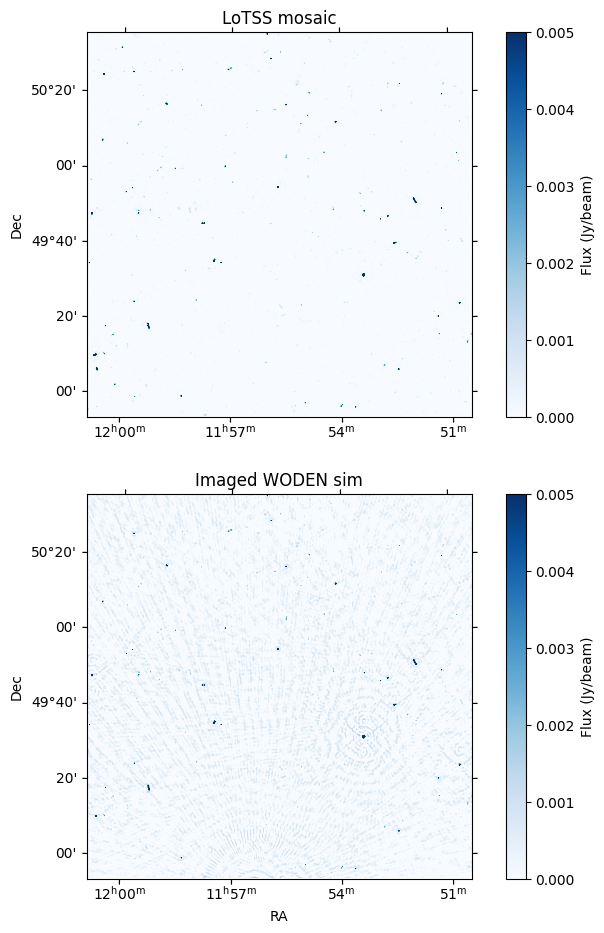
OK, so obviously the CLEAN on the WODEN sim isn’t the greatset. This image is not beam corrected, so sources towards the edge of the field appear dimmer. And of course I cropped the sky model to the cutout size, so we’re missing some sources from the corners. But overall I reckon this is a decent example of what you can do, and we’re matching reality pretty well.