Primary Beams

WODEN has been written to include stationary primary beams. That means the beam is pointed at a constant azimuth / zenith angle during an observation. There are currently three primary beams available, which are detailed below.

MWA Fully Embedded Element

The Murchison Widefield Array (MWA, Tingay et al. 2013) has 16 bow-tie dipoles arranged in a 4 by 4 grid as recieving elements, yielding a grating-lobe style primary beam.

WODEN incudes a GPU-implementation of the MWA Fully Embedded Element (FEE) Beam pattern (Sokolowski et al. 2017), which to date is the most accurate model of the MWA primary beam. This model is defined in a spherical harmonic coordinate system, which is polarisation-locked to instrumental azimuth / elevation coordinates. WODEN however uses Stokes parameters to define it’s visibilities, and so a rotation of the beam about parallactic angle (as calculated using erfa) is applied to align the FEE beam to move it into the Stokes frame.

Due to convention issues with whether ‘X’ means East-West or North-South, and whether azimuth starts towards North and increase towards East, we also find is necessary to reorder outputs and apply a sign flip to two of the outputs of the MWA FEE code. For an exhaustive investigation into why this is necessary to obtain the expected Stokes parameters, see polarised_source_and_FEE_beam.ipynb which lives here

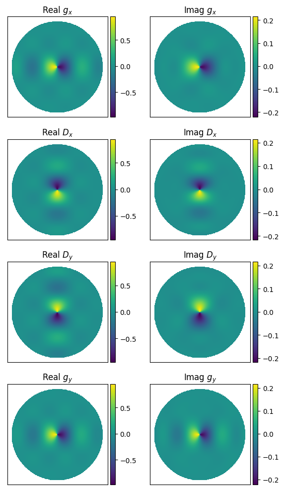
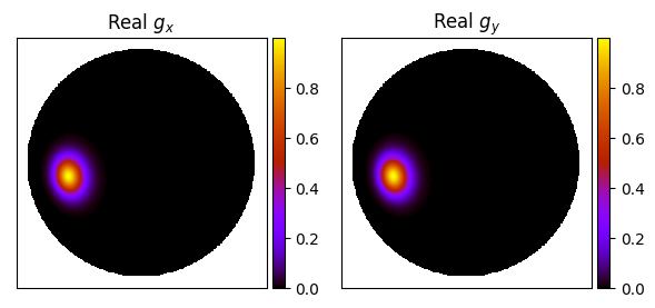
I can define the Jones matrix of the primary beam as:

\[\begin{split}\mathbf{J_\mathrm{linear}} = \begin{bmatrix} g_{x} & D_{x} \\ D_{y} & g_{y} \\ \end{bmatrix}.\end{split}\]

Here, the subscript \(x\) means a polarisation angle of \(0^\circ\) and \(y\) an angle of \(90^\circ\), \(g\) means a gain term, and \(D\) means a leakage term (so \(x\) means North-South and \(y\) is East-West). Under this definition, a typical zenith-pointing looks like this:

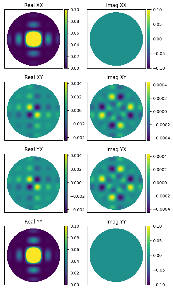
These plots are all sky, with northward at the top. If we assume the sky is totally Stokes I, this will yield instrumental polarisations (where ‘XX’ is North-South and ‘YY’ is East-West) like this:

The MWA beam is electronically steered, which can be defined via integer delays and supplied to the MWA FEE beam. run_woden.py can read these directly from an MWA metafits file, or can be directly supplied using the --MWA_FEE_delays argument.

Warning

The frequency resolution of the MWA FEE model is 1.28 MHz. I have NOT yet coded up a frequency interpolation, so the frequency response for a given direction looks something like the below. This is coming in the future.

In fact, when running using the MWA FEE band, I only calculate the beam response once per coarse band. If you set your --coarse_band_width to greater than 1.28 MHz you’ll make this effect even worse. If you stick to normal MWA observational params (with the default 1.28 MHz) all will be fine.

EDA2

The 2nd version of the Engineering Development Array (EDA2, Wayth et al. 2017), is an SKA_LOW test station, which swaps the planned logarithmic ‘christmas tree’ dipoles for MWA bow-tie dipoles. Currently, WODEN just assumes a perfect dipole with an infinite ground screen as a beam model. This makes the primary beam entirely real, with no leakage terms. Explicitly, the beam model is

\[\begin{split}\mathcal{G} = 2\sin\left(\pi \frac{2h}{\lambda} \cos(\theta) \right) \\ g_x = \mathcal{G}\arccos\left(\sin(\theta)\cos(\phi)\right) \\ g_y = \mathcal{G}\arccos\left(\sin(\theta)\sin(\phi)\right)\end{split}\]

where \(h\) is the height of the dipole, \(\lambda\) is the wavelength, \(\theta\) is the zenith angle, \(\phi\) is the azimuth angle. I’ve set \(h=0.3\) m.

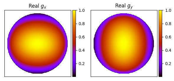
The beams basically see the whole sky (this image shows some \(\mathbf{J_\mathrm{linear}}\) values at 70 MHz):

Note

The EDA2 beam is neither physically nor electronically steered, so it always points towards zenith.

Gaussian

This is a toy case of a symmetric (major = minor) Gaussian primary beam. The beam gets smaller on the sky with increasing frequency, but both polarisations are identical. You can control the pointing of the beam (which remains constant in az/za for a single observation) via an initial RA/Dec pointing (--gauss_ra_point, --gauss_dec_point), and the FWHM of the beam (--gauss_beam_FWHM) at a reference frequency (--gauss_beam_ref_freq).

I’ve implemented this beam by creating a cosine angle coordinate system locked to the initial hour angle and declination of the specified RA,Dec pointing \(l_\mathrm{beam}, m_\mathrm{beam}, n_\mathrm{beam}\). The beam is then calculated as

\[G(l_\mathrm{beam}, m_\mathrm{beam}) = \exp \left( -\left( al_\mathrm{beam}^2 + 2bl_\mathrm{beam}m_\mathrm{beam} + cm_\mathrm{beam}^2 \right) \right)\]

where

\[\begin{split}a = \frac{\cos(\phi_{\mathrm{PA}})^2}{2\sigma_l^2} + \frac{\sin(\phi_{\mathrm{PA}})^2}{2\sigma_m^2} \\ b = -\frac{\sin(2\phi_{\mathrm{PA}})}{4\sigma_l^2} + \frac{\sin(2\phi_{\mathrm{PA}})}{4\sigma_m^2} \\ c = \frac{\sin(\phi_{\mathrm{PA}})^2}{2\sigma_l^2} + \frac{\cos(\phi_{\mathrm{PA}})^2}{2\sigma_m^2}.\end{split}\]

Currently, I have set the position angle of the beam \(\phi_{\mathrm{PA}}=0\) the std \(\sigma_l = \sigma_m\) to be equal, as:

\[\sigma_l = \sigma_m = \frac{\sin(\varphi_0)}{ 2\sqrt{2\ln(2)} }\frac{\nu_0}{\nu}\]

where \(\varphi_0\) is the desired FWHM at reference frequency \(\nu_0\), and \(\nu\) is the frequency to calculate the beam at.

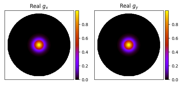
An example of a zenith pointing, with \(\varphi_0 = 10^\circ, \nu_0=100\) MHz looks like:

Using the same settings with an off-zenith pointing yields:

which at least visually looks like we are getting realistic-ish projection effects of the beam towards the horizon.

Note

The machinery is there to have different major / minor axes and a position angle if this is desired. Just open an issue on the github if you want this implemented.