Visibility Calculations

This section assumes a basic understanding on radio interferometry, assuming you know what visibilities and baselines are, and are familiar with the \(u,v,w\) and \(l,m,n\) coordinate systems. I can recommend Thompson, Moran, & Swenson 2017 if you are looking to learn / refresh these concepts. This section is basically a copy/paste from Line et al. 2020.

Note

In Line et al. 2020, I detailed that I was using the atomicAdd functionality in CUDA. This is no longer true, as I’ve found a loop inside my kernels is actually faster than being fully parallel and using atomicAdd. The calculations being made have remained the same.

Measurement Equation and Point Sources

WODEN analytically generates a sky model directly in visibility space via the measurement equation (c.f. Thompson, Moran, & Swenson 2017)

\[V(u,v,w) = \int \mathcal{B}(l,m) I(l,m) \exp[-2\pi i(ul + vm + w(n-1))] \dfrac{dldm}{n},\]

where \(V(u,v,w)\) is the measured visibility at baseline coordinates \(u,v,w\), given the sky intensity \(\mathcal{S}(l,m)\) and instrument beam pattern \(\mathcal{B}(l,m)\), which are functions of the direction cosines \(l,m\), with \(n=\sqrt{1-l^2-m^2}\). This can be discretised for point sources such that

\[V(u_i,v_i,w_i) = \sum_j \mathcal{B}(l_j,m_j)\mathcal{S}(l_j,m_j) \exp[-2\pi i(u_il_j + v_im_j + w_i(n_j-1))],\]

where \(u_i,v_i,w_i\) are the visibility co-ordinates of the \(i^{\mathrm{th}}\) baseline, and \(l_j\), \(m_j\), \(n_j\) is the sky position of the \(j^{\mathrm{th}}\) point source.

\(\mathcal{S}(l,m)\) includes all the Stokes parameters \(I, Q, U, V\) in WODEN, with these parameters extrapolated from an input catalogue, along with the position on the sky. \(u,v,w\) are set by a supplied array layout, phase centre, and location on the Earth.

Note

\(u_i,v_i,w_i\), \(\mathcal{S}\), and \(\mathcal{B}\) are also functions of frequency, so must be calculated for each frequency steps as required.

Gaussian and Shapelet sources

You can inject morphology into your sources analytically by tranforming a visibility into a Gaussian or Shapelet source. We utilise the RTS methodology of inserting a visibility “envelope” \(\xi\) into the visibility equation:

\[V(u_i,v_i,w_i) = \sum_j \xi_j(u_i,v_i)\mathcal{B}(l_j,m_j)\mathcal{S}(l_j,m_j) \exp[-2\pi i(u_il_j + v_im_j + w_i(n_j-1))],\]

For a Gaussian, this envelope looks like

\[\begin{split}\begin{align} &\xi_j = \exp\left( -\dfrac{\pi^2}{4\ln(2)} \left( k_x^2\theta_\mathrm{maj}^2 + k_y^2\theta_\mathrm{min}^2\right) \right); \\ &k_x = \cos(\phi_{\textrm{PA}})v_i + \sin(\phi_{\textrm{PA}})u_i; \\ &k_y = -\sin(\phi_{\textrm{PA}})v_i + \cos(\phi_{\textrm{PA}})u_i; \end{align}\end{split}\]

where \(\theta_\mathrm{maj}\) and \(\theta_\mathrm{min}\) are the major and minor axes and \(\phi_{\textrm{PA}}\) the position angle of an elliptical Gaussian.

For a shapelet model, the envelope looks like:

\[\begin{split}\begin{align} &\xi_j = \sum^{p_k +p_l < p_\mathrm{max}}_{k,l} C_{p_k,p_l} \tilde{B}_{p_k,p_l}(k_x,k_y); \label{eq:shape-env} \\ &k_x = \dfrac{\pi}{\sqrt{2\ln(2)}} \left[\cos(\phi_{PA})v_{i,j} + \sin(\phi_{PA})u_{i,j} \right]; \label{eq:scale-shape-x} \\ &k_y = \dfrac{\pi}{\sqrt{2\ln(2)}} \left[-\sin(\phi_{PA})v_{i,j} + \cos(\phi_{PA})u_{i,j} \right], \label{eq:scale-shape-y} \end{align}\end{split}\]

where \(u_{i,j},v_{i,j}\) are visibility co-ordinates for baseline \(i\), calculated with a phase-centre \(RA_j,\delta_j\), which corresponds to the central position \(x_0,y_0\) used to fit the shapelet model in image-space. The shapelet basis function values \(\tilde{B}_{p_k,p_l}(u,v)\) can be calculated by interpolating from one dimensional look-up tables of \(\tilde{B}(k_x;1)\), and scaling by the appropriate \(\beta\) (c.f. Equation 1 in Line et al. 2020 - see for a introduction and breakdown of shapelets bais functions).

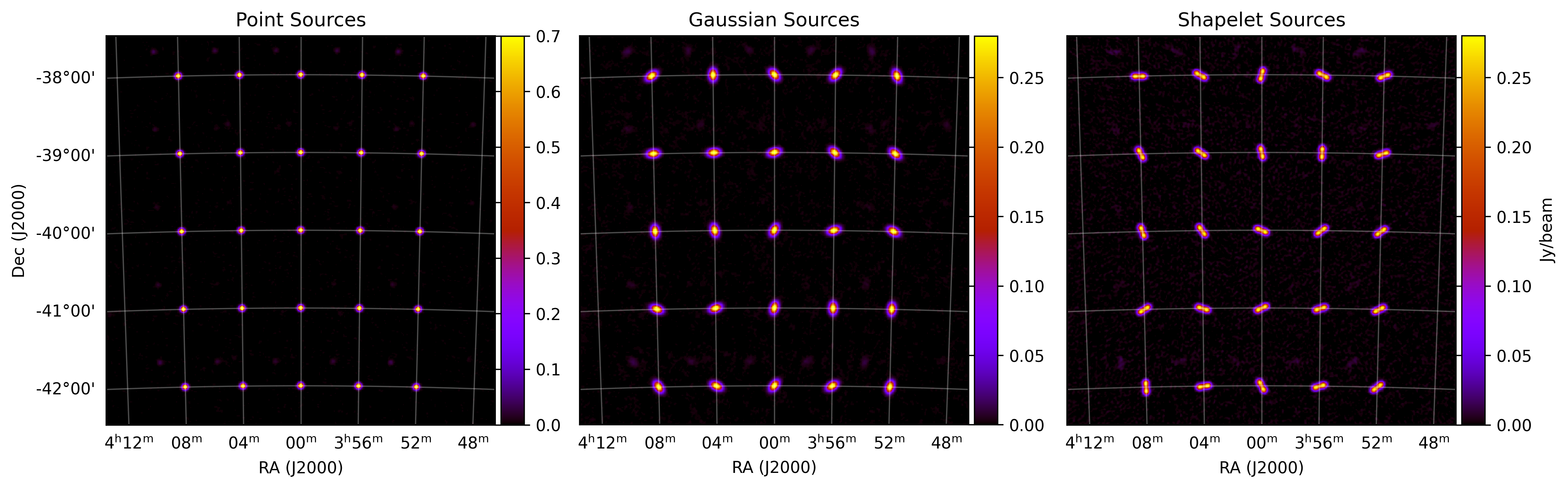
You can see the difference between the three types of sky model component below. You can generate this plot yourself, checkout the section Grid Component Models.