HERA simulations

We use pyuvdata.UVBeam to calculate the HERA primary beam. There are a number of input data formats UVBeam can read. So far, WODEN has options to reads in CST text files, and a beam model FITS format. We’ll use examples of both of these formats here, grabbing random examples from various HERA-related repositories. We’ll look at the primary beam patters, and then run an end-to-end simulation using the HERA beam model.

Primary beam patterns

The UVBeam wrapper inside WODEN is designed to read in RA,Dec coords from a sky catalogue, so let’s make a grid of az,za and convert them to RA,Dec coords at the HERA location. We’ll grab that from pyuvdata:

from pyuvdata.telescopes import known_telescope_location

##this is an astropy location object
location = known_telescope_location("HERA")

latitude = location.lat.value
longitude = location.lon.value
height = location.height.value
print(f"Latitude: {latitude} degrees")
print(f"Longitude: {longitude} degrees")
print(f"Height: {height} m")

Latitude: -30.72152612068926 degrees
Longitude: 21.42830382686301 degrees
Height: 1051.6900000007606 m

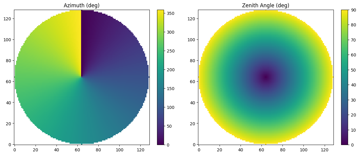
Make the az/za grid:

import numpy as np
import matplotlib.pyplot as plt

nside = 129
xrange = np.linspace(-1, 1, nside)
yrange = np.linspace(-1, 1, nside)
xcoords, ycoords = np.meshgrid(xrange, yrange)

za = np.sqrt(xcoords**2 + ycoords**2)*np.pi/2
az = np.pi/2 - np.arctan2(ycoords, xcoords)

az[az < 0] += 2*np.pi

below_horizon = za > np.pi/2
az[below_horizon] = np.nan
za[below_horizon] = np.nan

fig, axs = plt.subplots(1,2, figsize=(12, 5), layout='constrained') 

im = axs[0].imshow(np.degrees(az), origin='lower')
plt.colorbar(im, ax=axs[0])
im = axs[1].imshow(np.degrees(za), origin='lower')
plt.colorbar(im, ax=axs[1])
axs[0].set_title('Azimuth (deg)')
axs[1].set_title('Zenith Angle (deg)')
plt.show()

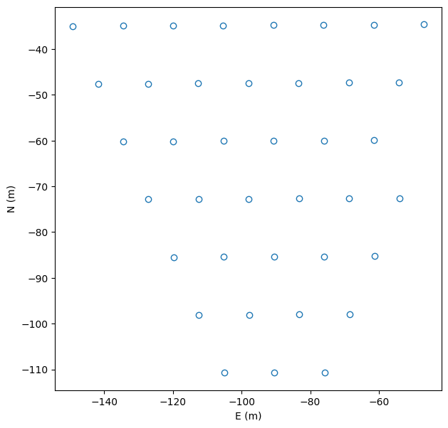
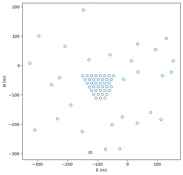
Now convert to RA,Dec coords. For that we need an observing time. We’ll be using the HERA phase 1 array layout, so let’s pick a date in between Oct 2017 and April 2018, when phase 1 was being used (Abdurashidova et al.). They also used three field centres. Let’s pick F1 which is centred at RA=2h:

from astropy.time import Time

obstime = Time("2017-11-11T21:09:30", scale='utc', location=location)

lst_deg = obstime.sidereal_time('apparent').to_value('deg')
print(f"LST: {lst_deg} degrees")

LST: 30.001385332537474 degrees

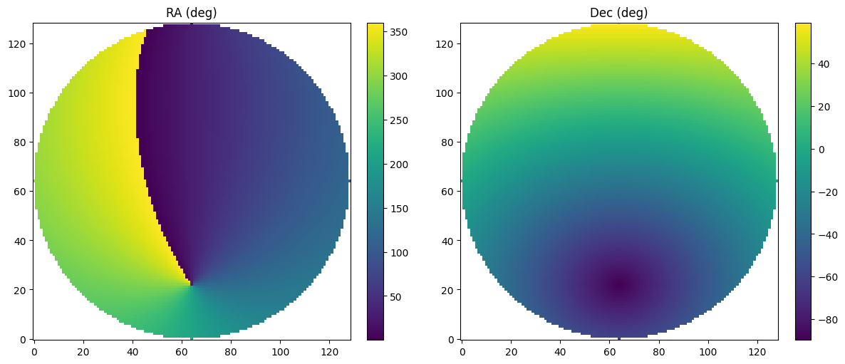
An LST of 30 deg (two hours) is what we want so this is close enough. Righto, now we can convert the az,za grid to RA,Dec coords:

import erfa

has, decs = erfa.ae2hd(az, np.pi/2-za, np.radians(latitude))

ras = np.radians(lst_deg) - has

ras[ras < 0] += 2*np.pi  # wrap RA to [0, 2pi]

fig, axs = plt.subplots(1,2, figsize=(12, 5), layout='constrained') 

im = axs[0].imshow(np.degrees(ras), origin='lower')
plt.colorbar(im, ax=axs[0])
im = axs[1].imshow(np.degrees(decs), origin='lower')
plt.colorbar(im, ax=axs[1])
axs[0].set_title('RA (deg)')
axs[1].set_title('Dec (deg)')
plt.show()

CST text files

After some online sleuthing, you can find some old CST files in Nicolas Fagnoni’s Simulations repo. Let’s download and unpack the 100 to 150 MHz files.

from glob import glob

files = glob("hera_beam/*.txt")

files.sort()


with open("hera_cst_4.9m_pattern_list.txt", "w") as f:

    for file in files:
        freq = file.split("_")[-1].split("MHz")[0]
        
        f.write(f"{file},{freq}\n")

%%bash
# Download the HERA E-field pattern

mkdir -p hera_beam

wget "https://github.com/Nicolas-Fagnoni/Simulations/raw/refs/heads/master/Radiation%20patterns/Archive/E-field%20pattern%20-%20Rigging%20height%204.9%20m/HERA_4.9m_E-pattern_100-150MHz.zip" -O hera_beam/HERA_4.9m_E-pattern_100-150MHz.zip

unzip hera_beam/HERA_4.9m_E-pattern_100-150MHz.zip -d hera_beam

Beam pattern names come out with spaces in them, annoying for Linux systems, so I’m going to rename them here

from subprocess import call
from glob import glob

files = glob("hera_beam/*.txt")
    
for ind in range(len(files)):
    cmd = f"mv '{files[ind]}' {''.join(files[ind].split(' '))}"
    # print(cmd)
    call(cmd, shell=True)

First of all, we make a UVBeam object from the CST text files. To do that, need a list of all the filenames, and an array of associated frequencies.

from wodenpy.primary_beam.use_uvbeam import setup_HERA_uvbeams_from_CST

cst_files = sorted(glob("hera_beam/*.txt"))
cst_freqs = [float(file.split("_")[-1].split("MHz")[0])*1e+6 for file in cst_files]

uvbeam_objs = setup_HERA_uvbeams_from_CST(cst_files, cst_freqs)

Finally let calculate the beam pattern. We’ll do two time steps and two frequencies. The HERA beam is zenith-locked. As we’re feeding in RA,Dec coords, we should see the beam pattern centred in the first time step, and then shifted away from centred in the second time step.

from wodenpy.primary_beam.use_uvbeam import run_uvbeam

##no need to do precession for simple test here
j2000_latitudes = np.radians([latitude]*2)
##add an extra 2 hours to lst for second time step
j2000_lsts = np.radians([lst_deg, lst_deg + 60.0])

freqs = np.array([100e+6, 150e+6])

all_jones_cst = run_uvbeam(uvbeam_objs, ras.flatten(), decs.flatten(),
                           j2000_latitudes, j2000_lsts,
                           freqs, iau_order=True, parallactic_rotate=True)

invalid value encountered in hd2ae

Let’s make some beam plots. I’m going to log the amplitudes to make the pattern more visible. run_uvbeam has been written to make outputs that fit into the wodenpy beam framework, which can handle unique beam models per station. The beam models I’m using here are only for one station, so if you see me setting station=0, that’s why.

def plot_jones(all_jones, time_ind, lsts, freq_ind, freqs, title, nside):
    
    fig, axs = plt.subplots(4, 4, figsize=(12, 10), layout='constrained')
    
    station_ind=0
    
    gx = all_jones[0, time_ind, freq_ind, :, 0, 0]
    Dx = all_jones[0, time_ind, freq_ind, :, 1, 0]
    Dy = all_jones[0, time_ind, freq_ind, :, 0, 1]
    gy = all_jones[0, time_ind, freq_ind, :, 1, 1]
    
    ax = 0
    for pol, label in zip([gx, Dx, Dy, gy], ['gx', 'Dx', 'Dy', 'gy']):
        
        pol = pol.reshape((nside, nside))
        
        im = axs[ax, 0].imshow(np.real(pol), origin='lower')
        axs[ax, 0].set_title(f'Real {label}')
        plt.colorbar(im, ax=axs[ax, 0])
        im = axs[ax, 1].imshow(np.imag(pol), origin='lower')
        axs[ax, 1].set_title(f'Imag {label}')
        plt.colorbar(im, ax=axs[ax, 1])
        im = axs[ax, 2].imshow(np.log10(np.abs(pol)), origin='lower')
        axs[ax, 2].set_title(f'log 10 abs {label}')
        plt.colorbar(im, ax=axs[ax, 2])
        im = axs[ax, 3].imshow(np.angle(pol), origin='lower')
        axs[ax, 3].set_title(f'Phase {label}')
        plt.colorbar(im, ax=axs[ax, 3])
        
        ax += 1
        
    for ax in axs.flat:
        ax.set_xticks([])
        ax.set_yticks([])
        
    plt.suptitle(f'{title} {freqs[freq_ind]/1e+6:.1f} MHz, LST {np.degrees(lsts[time_ind]):.1f} deg')
    plt.show()
    
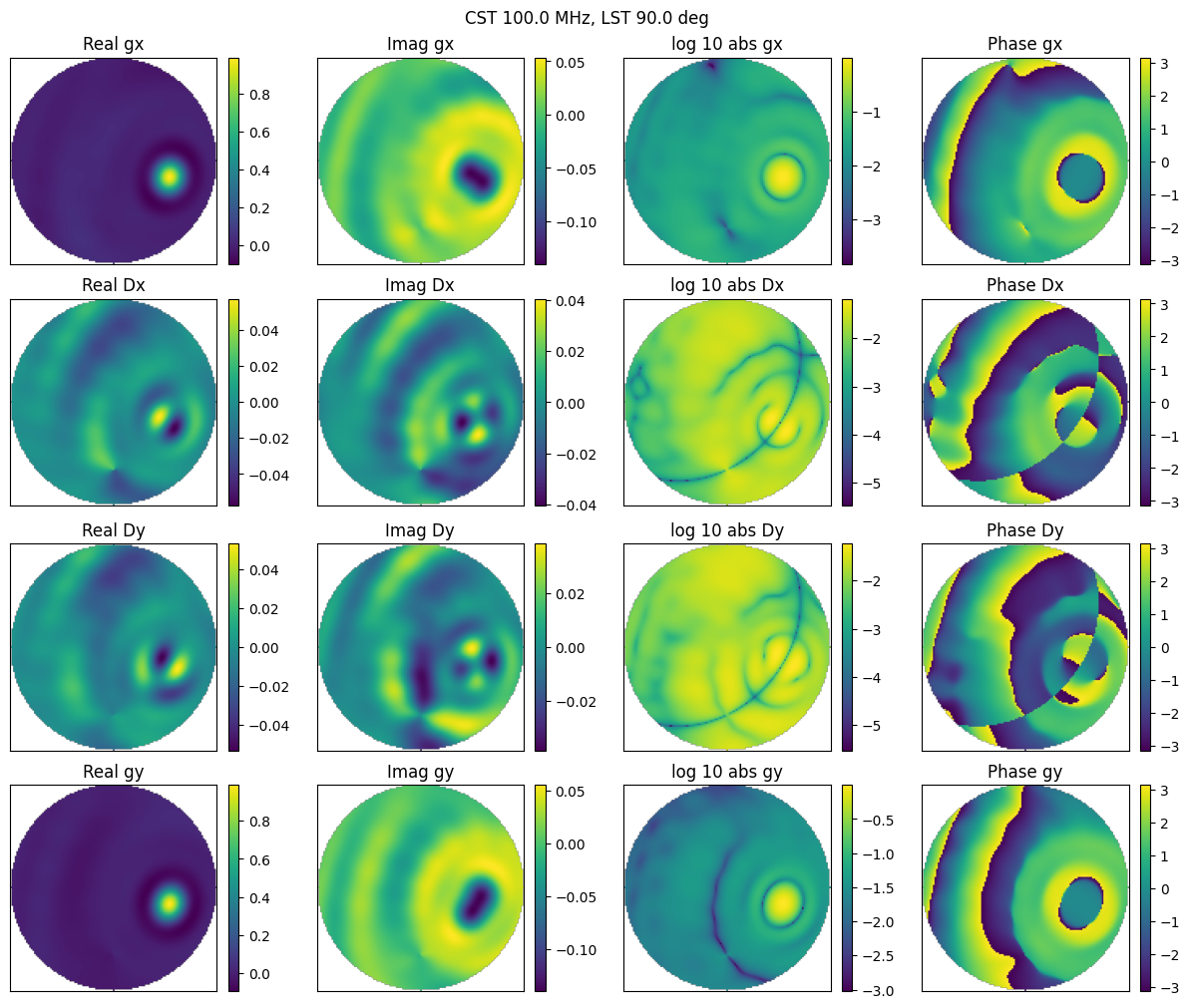
plot_jones(all_jones_cst, 0, j2000_lsts, 0, freqs, 'CST', nside)

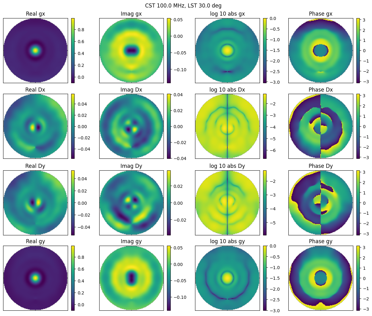
Looks pretty single dipole-like. I’ve set iau_order=True as internally WODEN uses the IAU conventions. This means gx in above is the gain term for the north-south dipole. That means gx should be more sensitive to the east-west. The beam pattern does look elongated in the east-west direction, and vice-versa for gy, so the polarisations are behaving as expected. Let’s check the beam gets smaller at higher frequencies, and moves with time.

plot_jones(all_jones_cst, 0, j2000_lsts, 1, freqs, 'CST', nside)

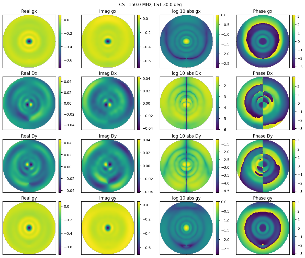
plot_jones(all_jones_cst, 1, j2000_lsts, 0, freqs, 'CST', nside)

Indeed it does, so things are looking good. Now let’s try the FITS format.

FITS beam file

We’ll do the same again but with a beam FITS format. Again, I’ve stalked HERA-repos, and found a FITS beam file in mativs which we can download.

%%bash

wget "https://github.com/HERA-Team/matvis/raw/refs/heads/main/src/matvis/data/NF_HERA_Dipole_small.fits" -O NF_HERA_Dipole_small.fits

from wodenpy.primary_beam.use_uvbeam import setup_HERA_uvbeams_from_single_file

uvbeam_fits_objs = setup_HERA_uvbeams_from_single_file("NF_HERA_Dipole_small.fits")

print(uvbeam_fits_objs[0].freq_array)

[1.00e+08 1.01e+08]

Unforntunately, this only contains two frequencies. By default, UVBeam wants to interpolate over frequencies, and the default interp needs three at a minimum. The WODEN wrapper will just switch interpolation off if there’s <3 frequencies. At least we can compare the beam patterns at 100MHz.

all_jones_fits = run_uvbeam(uvbeam_fits_objs, ras.flatten(), decs.flatten(),
                           j2000_latitudes, j2000_lsts,
                           freqs, iau_order=True, parallactic_rotate=True)

2025-06-02 11:15:17 - WARNING - Number of frequencies in the UVBeam object is less than 3.
WODEN will proceed, but will switch off frequency interpolation.
UVBeam needs at least three frequencies to perform default interpolation.
Further warnings of this type will be suppressed.

2025-06-02 11:15:17 - WARNING - Number of frequencies in the UVBeam object is less than 3.
WODEN will proceed, but will switch off frequency interpolation.
UVBeam needs at least three frequencies to perform default interpolation.
Further warnings of this type will be suppressed.

2025-06-02 11:15:17 - WARNING - Number of frequencies in the UVBeam object is less than 3.
WODEN will proceed, but will switch off frequency interpolation.
UVBeam needs at least three frequencies to perform default interpolation.
Further warnings of this type will be suppressed.

2025-06-02 11:15:17 - WARNING - Number of frequencies in the UVBeam object is less than 3.
WODEN will proceed, but will switch off frequency interpolation.
UVBeam needs at least three frequencies to perform default interpolation.
Further warnings of this type will be suppressed.

invalid value encountered in hd2ae

We can at least check that the beam moves with time; obviously it won’t change with frequency.

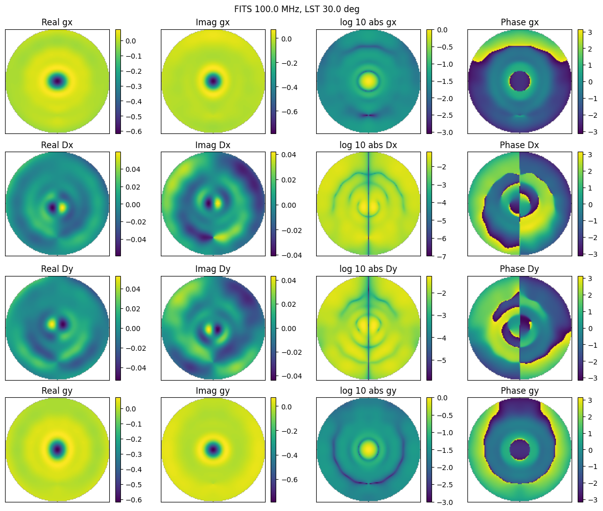
plot_jones(all_jones_fits, 0, j2000_lsts, 0, freqs, 'FITS', nside)

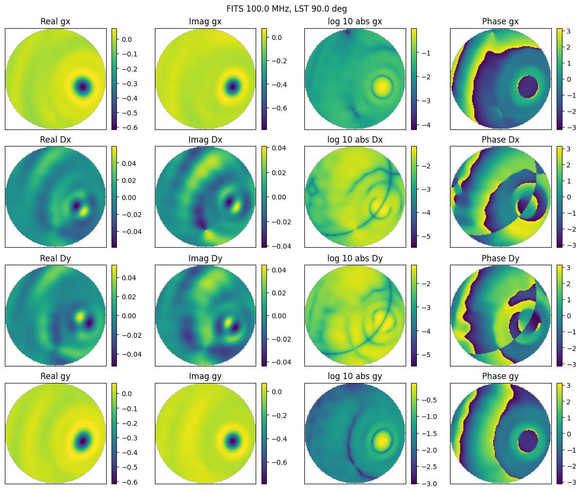
plot_jones(all_jones_fits, 1, j2000_lsts, 0, freqs, 'FITS', nside)

Let’s compare the gains of the two models at 100MHz to convince ourselves we’re plottings two different models.

fig, axs = plt.subplots(2, 3, figsize=(14, 10), layout='constrained')
    
station_ind=0
time_ind = 0
freq_ind = 0

gx_cst = all_jones_cst[station_ind, time_ind, freq_ind, :, 0, 0]
gx_fits = all_jones_fits[station_ind, time_ind, freq_ind, :, 0, 0]

gy_cst = all_jones_cst[station_ind, time_ind, freq_ind, :, 1, 1]
gy_fits = all_jones_fits[station_ind, time_ind, freq_ind, :, 1, 1]


for ind, pol, label in zip(range(6), [gx_cst, gx_fits, np.abs(gx_fits) - np.abs(gx_cst),
                                      gy_cst, gy_fits, np.abs(gy_fits) - np.abs(gy_cst)],
                                     ['gx CST', 'gx FITS', 'gx FITS - gx CST',
                                      'gy CST', 'gy FITS', 'gy FITS - gy CST']):
    
    pol = pol.reshape((nside, nside))
    
    col = ind % 3
    row = ind // 3
    im = axs[row, col].imshow(np.log10(np.abs(pol)), origin='lower')
    # im = axs[row, col].imshow(np.abs(pol), origin='lower')
    axs[row, col].set_title(f'{label}')
    plt.colorbar(im, ax=axs[row, col])
    
    
    
for ax in axs.flat:
    ax.set_xticks([])
    ax.set_yticks([])
    
plt.suptitle(f'Beam amplitude comparison (everything in log10 scale)')
plt.show()

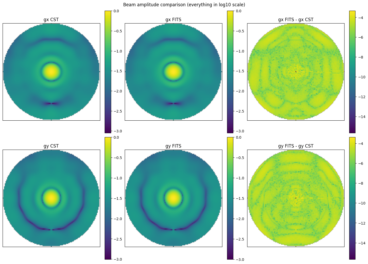
Huh well maybe these are actually the same model, just stored in different formats. There is a slight difference, so at least we’re defo reading in two different things, and they both work.

End-to-end simulation

Now let’s run an end-to-end simulation using the HERA beam model. We’ll use the CST text files, as they have more frequencies than the FITS file. I’m also going to just use the Aussie MWA sky model, as that’s already in the WODEN format, and HERA sits at almost the same latitude as the MWA.

Array layouts

I need an array lay however, so once again let’s get something off the interwebs:

import pandas as pd

url = "https://raw.githubusercontent.com/HERA-Team/hera_sim/main/src/hera_sim/data/tutorials_data/visibility_simulator/antenna_layout_hera_phase1.csv"
df = pd.read_csv(url, delimiter="\t")
df.head()

	Name	Number	BeamID	E	N	U
0	ANT0	0	0.0	-105.035302	-110.722053	0.938171
1	ANT1	1	0.0	-90.427459	-110.666264	0.928396
2	ANT2	2	0.0	-75.819616	-110.610476	0.918587
3	ANT11	11	0.0	-112.387519	-98.103144	0.788253
4	ANT12	12	0.0	-97.779676	-98.047355	0.718495

import numpy as np

num_ants = df.shape[0]

enh = np.empty((num_ants, 3), dtype=float)

enh[:, 0] = df["E"].values
enh[:, 1] = df["N"].values
enh[:, 2] = df["U"].values

Let’s have a look-see.

import matplotlib.pyplot as plt

fig, ax = plt.subplots(1, 1, figsize=(7,7))

ax.plot(enh[:, 0], enh[:, 1], 'o', mfc='none', label='HERA Phase 1 Antennas')

ax.set_xlabel('E (m)')
ax.set_ylabel('N (m)')

plt.show()

Save it to a format that WODEN can read.

np.savetxt('hera_phase1_antenna_layout.txt', enh,  fmt='%f', delimiter=' ')

Let’s make a version with some outrigger dishes so we can make some better images from the resultant simulation.

num_extra_ants = 30

enh_enhanced = np.zeros((num_ants + num_extra_ants, 3), dtype=float)
# # print(enh_enhanced.shape, enh.shape)

enh_enhanced[num_extra_ants:, :] = enh

east_mid = np.mean(enh[:, 0])
north_mid = np.mean(enh[:, 1])

radius = np.random.uniform(70, 300, num_extra_ants)
theta = np.random.uniform(0, 2 * np.pi, num_extra_ants)

enh_enhanced[:num_extra_ants, 0] = east_mid + radius * np.cos(theta)
enh_enhanced[:num_extra_ants, 1] = north_mid + radius * np.sin(theta)

            
np.savetxt('hera_phase1_antenna_layout_with_out-riggers.txt', enh_enhanced,  fmt='%f', delimiter=' ')

fig, ax = plt.subplots(1, 1, figsize=(7,7))

ax.plot(enh_enhanced[:, 0], enh_enhanced[:, 1], 'o', mfc='none', label='HERA Phase 1 Antennas + outriggers')

ax.set_xlabel('E (m)')
ax.set_ylabel('N (m)')

plt.show()

To make things tidy when running run_woden.py, I’ve setup the function to read in the CST files path and associated frequencies from a single csv file. Let’s write that now:

with open("hera_cst_4.9m_pattern_list.csv", "w") as f:
    for freq in range(100, 151, 1):
        f.write(f"hera_beam/HERA_4.9m_E-pattern_{freq}MHz.txt,{freq}e+6\n")

Now we need the sky model, so let’s download that:

%%bash

wget "https://github.com/JLBLine/srclists/raw/refs/heads/master/srclist_pumav3_EoR0LoBES_EoR1pietro_CenA-GP_2023-11-07.fits" -O srclist_pumav3_EoR0LoBES_EoR1pietro_CenA-GP_2023-11-07.fits

Now we have everything we need, let’s run a simulation. I’ll use frequency and time settings as specified in Abdurashidova et al.. I’m going to run the simulation using the outrigger dishes to make a better image.

%%bash

run_woden.py \
    --ra0=30.0 --dec0=-30.0 \
    --num_freq_channels=10 --num_time_steps=10 \
    --date=2017-11-11T21:09:30 --lowest_channel_freq=100e+6 \
    --freq_res=97.66e+3 --time_res=10.7 \
    --cat_filename=srclist_pumav3_EoR0LoBES_EoR1pietro_CenA-GP_2023-11-07.fits \
    --array_layout=hera_phase1_antenna_layout_with_out-riggers.txt \
    --band_nums=1 \
    --output_uvfits_prepend=woden_HERA+outriggers_F1 \
    --primary_beam=uvbeam_HERA \
    --num_threads=1 \
    --cst_file_list=hera_cst_4.9m_pattern_list.csv

/home/jack-line/software/WODEN_dev/woden_dev/bin/run_woden.py:4: DeprecationWarning: pkg_resources is deprecated as an API. See https://setuptools.pypa.io/en/latest/pkg_resources.html
  __import__('pkg_resources').require('wodenpy==2.5.0')

2025-06-02 11:15:31 - INFO - 
                                              )  (              )  
                                  (  (     ( /(  )\ )        ( /(  
                                  )\))(   ')\())(()/(   (    )\()) 
                                 ((_)()\ )((_)\  /(_))  )\  ((_)\  
                                 _(())\_)() ((_)(_))_  ((_)  _((_) 
                                 \ \((_)/ // _ \ |   \ | __|| \| | 
                                  \ \/\/ /| (_) || |) || _| | .` | 
                                   \_/\_/  \___/ |___/ |___||_|\_| 
                                   
                                 You are using wodenpy version/git hash: a43c383
                                 
2025-06-02 11:15:31 - INFO - Input arguments after parsing:
                             	Phase centre: 30.00000, -30.00000 deg
                             	Array central latitude: -30.722 deg
                             	Array central longitude: 21.428 deg
                             	Array central height: 1051.690 m
                             	Lowest channel frequency: 100.000 MHz
                             	Channel frequency resolution: 97.660 kHz
                             	Coarse band bandwidth: 1.280 MHz
                             	Num channels per coarse band: 10
                             	Start date: 2017-11-11T21:09:30
                             	Time resolution: 10.7 (s)
                             	Num time steps: 10
                             	Have read 69 antenna positions from array layout file: hera_phase1_antenna_layout_with_out-riggers.txt
                             	Will write outputs to: /home/jack-line/software/WODEN_dev/examples/HERA_sim
2025-06-02 11:15:31 - INFO - Obs epoch initial LST was 30.0269410869 deg
2025-06-02 11:15:31 - INFO - Setting initial J2000 LST to 29.8314110058 deg
2025-06-02 11:15:31 - INFO - Setting initial mjd to 58068.8816591436
2025-06-02 11:15:31 - INFO - After precession initial latitude of the array is -30.8055128992 deg
2025-06-02 11:15:31 - INFO - Precessing array layout to J2000
2025-06-02 11:15:31 - INFO - Will create a HERA beam from CST files listed in this file:
                             	hera_cst_4.9m_pattern_list.csv
                             Have read the following frequencies from this file:
                             	[100000000.0, 101000000.0, 102000000.0, 103000000.0, 104000000.0, 105000000.0, 106000000.0, 107000000.0, 108000000.0, 109000000.0, 110000000.0, 111000000.0, 112000000.0, 113000000.0, 114000000.0, 115000000.0, 116000000.0, 117000000.0, 118000000.0, 119000000.0, 120000000.0, 121000000.0, 122000000.0, 123000000.0, 124000000.0, 125000000.0, 126000000.0, 127000000.0, 128000000.0, 129000000.0, 130000000.0, 131000000.0, 132000000.0, 133000000.0, 134000000.0, 135000000.0, 136000000.0, 137000000.0, 138000000.0, 139000000.0, 140000000.0, 141000000.0, 142000000.0, 143000000.0, 144000000.0, 145000000.0, 146000000.0, 147000000.0, 148000000.0, 149000000.0, 150000000.0]
2025-06-02 11:15:31 - INFO - Doing the initial mapping of sky model
2025-06-02 11:15:32 - INFO - Sky model mapping took 0.0 mins
2025-06-02 11:15:32 - INFO - Have read in 348067 components
2025-06-02 11:15:32 - INFO - After cropping there are 239552 components
2025-06-02 11:15:32 - INFO - Will load libwoden from /home/jack-line/software/WODEN_dev/wodenpy/libwoden_double.so
2025-06-02 11:15:32 - INFO - Creating UVBeam objects. This may take a while
2025-06-02 11:15:40 - INFO - UVBeam objects have been initialised
2025-06-02 11:15:40 - INFO - Running in serial on GPU.
                             Will read sky model using one thread (UVBeam models seem to do their own threading, trying to thread leads to GIL issues)
                             There are 1 sets of sky models to run
2025-06-02 11:15:40 - INFO - Reading (and calculating primary beam values for) set 0 sky models
2025-06-02 11:15:40 - INFO - From sky set 0 thread num 0 reading 225042 points, 14449 gauss, 61 shape, 10280 shape coeffs
2025-06-02 11:19:35 - INFO - Finshed sky set 0 reading thread num 0 in 234.6 seconds
2025-06-02 11:19:35 - INFO - Coverting sky model and beam values into `ctypes` for sky set 0
2025-06-02 11:21:00 - INFO - `ctype` catalogue for round 0 created in 84.9 seconds
2025-06-02 11:21:00 - INFO - Sending Sky set 0 to the GPU
2025-06-02 11:21:38 - INFO - Sky set 0 has returned from the GPU after 38.2 seconds
2025-06-02 11:21:39 - INFO - Have completed 249832 of 249832 components calcs (100.0%)
2025-06-02 11:21:39 - INFO - Full run took 0:06:08.165001
2025-06-02 11:21:39 - INFO - WODEN is done. Closing the log. S'later

Righto, we have a simulation! Let’s make an image

%%bash

woden_uv2ms.py \
  --uvfits_prepend=woden_HERA+outriggers_F1_band \
  --band_nums=1

/home/jack-line/software/WODEN_dev/woden_dev/bin/woden_uv2ms.py:4: DeprecationWarning: pkg_resources is deprecated as an API. See https://setuptools.pypa.io/en/latest/pkg_resources.html
  __import__('pkg_resources').require('wodenpy==2.5.0')
The telescope frame is set to '????', which generally indicates ignorance. Defaulting the frame to 'itrs', but this may lead to other warnings or errors.
antenna_diameters are not set or are being overwritten. antenna_diameters are set using values from known telescopes for HERA.
Writing in the MS file that the units of the data are uncalib, although some CASA process will ignore this and assume the units are all in Jy (or may not know how to handle data in these units).

%%bash 

wsclean -name woden_HERA+outriggers_F1 -size 2048 2048 -niter 3000 \
  -auto-threshold 0.5 -auto-mask 3 -pol I -multiscale \
  -weight uniform -scale 0.03 -j 12 -mgain 0.85 -no-update-model-required  \
  woden_HERA+outriggers_F1_band*.ms 

WSClean version 3.4 (2023-10-11)
This software package is released under the GPL version 3.
Author: André Offringa (offringa@gmail.com).

No corrected data in first measurement set: tasks will be applied on the data column.
=== IMAGING TABLE ===
       # Pol Ch JG ²G FG FI In Freq(MHz)
| Independent group:
+-+-J- 0  I   0  0  0  0  0  0  100-101 (10)
Reordering woden_HERA+outriggers_F1_band01.ms into 1 x 1 parts.
Reordering: 0%....10%....20%....30%....40%....50%....60%....70%....80%....90%....100%
Initializing model visibilities: 0%....10%....20%....30%....40%....50%....60%....70%....80%....90%....100%
 == Constructing PSF ==
Precalculating weights for uniform weighting...
Opening reordered part 0 spw 0 for woden_HERA+outriggers_F1_band01.ms
Detected 62.7 GB of system memory, usage not limited.
Opening reordered part 0 spw 0 for woden_HERA+outriggers_F1_band01.ms
Determining min and max w & theoretical beam size... DONE (w=[2.0881e-05:2.37788] lambdas, maxuvw=181.324 lambda)
Theoretic beam = 18.96'
Minimal inversion size: 468 x 468, using optimal: 480 x 480
Loading data in memory...
Gridding 23460 rows...
Gridded visibility count: 234600
Fitting beam... major=20.77', minor=17.3', PA=154.2 deg, theoretical=18.96'.
Writing psf image... DONE
 == Constructing image ==
Opening reordered part 0 spw 0 for woden_HERA+outriggers_F1_band01.ms
Loading data in memory...
Gridding 23460 rows...
Gridded visibility count: 234600
Writing dirty image...
 == Deconvolving (1) ==
Estimated standard deviation of background noise: 753.5 mJy
Scale info:
- Scale 0, bias factor=1, psfpeak=1, gain=0.1, kernel peak=0.00804104
- Scale 42, bias factor=1.7, psfpeak=0.20405, gain=0.490075, kernel peak=0.00217442
- Scale 84, bias factor=2.8, psfpeak=0.0405386, gain=2.46678, kernel peak=0.000590399
- Scale 169, bias factor=4.6, psfpeak=0.00572252, gain=17.4748, kernel peak=0.000154076
- Scale 337, bias factor=7.7, psfpeak=0.000980569, gain=101.982, kernel peak=3.93725e-05
- Scale 674, bias factor=12.9, psfpeak=0.000276781, gain=361.297, kernel peak=9.89861e-06
RMS per scale: {0: 875.31 mJy, 42: 313.63 mJy, 84: 175.54 mJy, 169: 138.51 mJy, 337: 131.24 mJy, 674: 120.36 mJy}
Starting multi-scale cleaning. Start peak=29.98 Jy, major iteration threshold=4.5 Jy
Iteration 3, scale 0 px : 22.01 Jy at 1092,1039
Iteration 8, scale 0 px : 17.45 Jy at 1022,994
Iteration 14, scale 0 px : 12.94 Jy at 1198,804
Iteration 21, scale 0 px : 10.14 Jy at 1023,994
Iteration 30, scale 0 px : 8.11 Jy at 897,807
Iteration 48, scale 0 px : 6.57 Jy at 1244,1144
Iteration 71, scale 0 px : 5.21 Jy at 1022,994
Subminor loop is near minor loop threshold. Initiating countdown.
(8) Iteration 89, scale 0 px : 4.47 Jy at 1082,1034
Minor loop finished, continuing cleaning after inversion/prediction round.
Assigning from 1 to 1 channels...
 == Converting model image to visibilities ==
Opening reordered part 0 spw 0 for woden_HERA+outriggers_F1_band01.ms
Predicting 23460 rows...
Writing...
 == Constructing image ==
Opening reordered part 0 spw 0 for woden_HERA+outriggers_F1_band01.ms
Loading data in memory...
Gridding 23460 rows...
Gridded visibility count: 234600
 == Deconvolving (2) ==
Estimated standard deviation of background noise: 496.13 mJy
Scale info:
- Scale 0, bias factor=1, psfpeak=1, gain=0.1, kernel peak=0.00804104
- Scale 42, bias factor=1.7, psfpeak=0.20405, gain=0.490075, kernel peak=0.00217442
- Scale 84, bias factor=2.8, psfpeak=0.0405386, gain=2.46678, kernel peak=0.000590399
- Scale 169, bias factor=4.6, psfpeak=0.00572252, gain=17.4748, kernel peak=0.000154076
- Scale 337, bias factor=7.7, psfpeak=0.000980569, gain=101.982, kernel peak=3.93725e-05
- Scale 674, bias factor=12.9, psfpeak=0.000276781, gain=361.297, kernel peak=9.89861e-06
RMS per scale: {0: 520.17 mJy, 42: 202.93 mJy, 84: 138.72 mJy, 169: 124.9 mJy, 337: 120.68 mJy, 674: 110.96 mJy}
Starting multi-scale cleaning. Start peak=4.48 Jy, major iteration threshold=1.49 Jy (final)
Iteration 126, scale 0 px : 3.66 Jy at 1101,1068
Iteration 183, scale 0 px : 2.92 Jy at 833,1245
Iteration 269, scale 42 px : 2.49 Jy at 1020,997
Iteration 274, scale 0 px : 2.36 Jy at 995,1003
Iteration 396, scale 0 px : 1.89 Jy at 834,1245
Iteration 594, scale 674 px : -1.79 Jy at 1679,1673
Subminor loop is near minor loop threshold. Initiating countdown.
(8) Iteration 605, scale 42 px : 1.48 Jy at 1020,997
Cleaning finished because the final threshold was reached.
Auto-masking threshold reached; continuing next major iteration with deeper threshold and mask.
Assigning from 1 to 1 channels...
 == Converting model image to visibilities ==
Opening reordered part 0 spw 0 for woden_HERA+outriggers_F1_band01.ms
Predicting 23460 rows...
Writing...
 == Constructing image ==
Opening reordered part 0 spw 0 for woden_HERA+outriggers_F1_band01.ms
Loading data in memory...
Gridding 23460 rows...
Gridded visibility count: 234600
 == Deconvolving (3) ==
Estimated standard deviation of background noise: 328.34 mJy
Scale info:
- Scale 0, bias factor=1, psfpeak=1, gain=0.1, kernel peak=0.00804104
- Scale 42, bias factor=1.7, psfpeak=0.20405, gain=0.490075, kernel peak=0.00217442
- Scale 84, bias factor=2.8, psfpeak=0.0405386, gain=2.46678, kernel peak=0.000590399
- Scale 169, bias factor=4.6, psfpeak=0.00572252, gain=17.4748, kernel peak=0.000154076
- Scale 337, bias factor=7.7, psfpeak=0.000980569, gain=101.982, kernel peak=3.93725e-05
- Scale 674, bias factor=12.9, psfpeak=0.000276781, gain=361.297, kernel peak=9.89861e-06
RMS per scale: {0: 334.71 mJy, 42: 113.62 mJy, 84: 61.03 mJy, 169: 46.58 mJy, 337: 43.46 mJy, 674: 39.8 mJy}
Starting multi-scale cleaning. Start peak=1.48 Jy, major iteration threshold=221.87 mJy
Iteration 755, scale 42 px : 1.31 Jy at 1020,997
Iteration 760, scale 0 px : 1.21 Jy at 995,1003
Iteration 932, scale 0 px : 991.62 mJy at 1022,987
Iteration 1120, scale 42 px : 896.86 mJy at 1020,997
Iteration 1125, scale 42 px : 690.13 mJy at 1020,997
Iteration 1130, scale 0 px : 825.07 mJy at 1014,1024
Iteration 1287, scale 0 px : 659.95 mJy at 1006,1148
Iteration 1493, scale 674 px : -569.96 mJy at 1679,1673
Iteration 1508, scale 0 px : -565.64 mJy at 1062,1021
Iteration 1597, scale 0 px : 460.04 mJy at 2040,960
Iteration 1800, scale 674 px : -415.25 mJy at 338,1709
Iteration 1809, scale 0 px : -372.67 mJy at 1062,1021
Iteration 1982, scale 42 px : 312.65 mJy at 1020,997
Iteration 1987, scale 674 px : -310.12 mJy at 378,520
Iteration 2002, scale 0 px : 297.77 mJy at 2040,960
Iteration 2157, scale 0 px : 241.11 mJy at 2040,960
Subminor loop is near minor loop threshold. Initiating countdown.
(8) Iteration 2226, scale 674 px : -223.2 mJy at 378,520
(7) Iteration 2227, scale 0 px : 221.71 mJy at 761,1054
Minor loop finished, continuing cleaning after inversion/prediction round.
Assigning from 1 to 1 channels...
 == Converting model image to visibilities ==
Opening reordered part 0 spw 0 for woden_HERA+outriggers_F1_band01.ms
Predicting 23460 rows...
Writing...
 == Constructing image ==
Opening reordered part 0 spw 0 for woden_HERA+outriggers_F1_band01.ms
Loading data in memory...
Gridding 23460 rows...
Gridded visibility count: 234600
 == Deconvolving (4) ==
Estimated standard deviation of background noise: 255.3 mJy
Scale info:
- Scale 0, bias factor=1, psfpeak=1, gain=0.1, kernel peak=0.00804104
- Scale 42, bias factor=1.7, psfpeak=0.20405, gain=0.490075, kernel peak=0.00217442
- Scale 84, bias factor=2.8, psfpeak=0.0405386, gain=2.46678, kernel peak=0.000590399
- Scale 169, bias factor=4.6, psfpeak=0.00572252, gain=17.4748, kernel peak=0.000154076
- Scale 337, bias factor=7.7, psfpeak=0.000980569, gain=101.982, kernel peak=3.93725e-05
- Scale 674, bias factor=12.9, psfpeak=0.000276781, gain=361.297, kernel peak=9.89861e-06
RMS per scale: {0: 260.15 mJy, 42: 85.56 mJy, 84: 41.42 mJy, 169: 27.48 mJy, 337: 23.61 mJy, 674: 20.93 mJy}
Starting multi-scale cleaning. Start peak=392 mJy, major iteration threshold=127.65 mJy (final)
Iteration 2241, scale 0 px : -360.76 mJy at 2043,1918
Iteration 2244, scale 0 px : -287.91 mJy at 1988,1012
Iteration 2272, scale 674 px : 294.7 mJy at 338,1709
Iteration 2285, scale 674 px : 221.17 mJy at 338,1709
Iteration 2299, scale 0 px : 261.88 mJy at 931,893
Iteration 2417, scale 0 px : 210.65 mJy at 727,1061
Iteration 2601, scale 0 px : -188.64 mJy at 1022,998
Iteration 2725, scale 42 px : 199.67 mJy at 1020,997
Iteration 2730, scale 42 px : 153.64 mJy at 1020,997
Subminor loop is near minor loop threshold. Initiating countdown.
(8) Iteration 2734, scale 0 px : -229.67 mJy at 1022,998
Iteration 2737, scale 0 px : -167.43 mJy at 1022,998
Iteration 2844, scale 674 px : 182.07 mJy at 338,1709
Iteration 2858, scale 674 px : 136.61 mJy at 338,1709
(7) Iteration 2861, scale 42 px : 188.13 mJy at 1020,997
Iteration 2866, scale 42 px : 144.77 mJy at 1020,997
(6) Iteration 2869, scale 0 px : -189.98 mJy at 1022,998
Iteration 2873, scale 0 px : 148.66 mJy at 1014,1024
(5) Iteration 2995, scale 0 px : 127.55 mJy at 1197,1067
Cleaning finished because the final threshold was reached.
Assigning from 1 to 1 channels...
Writing model image...
 == Converting model image to visibilities ==
Opening reordered part 0 spw 0 for woden_HERA+outriggers_F1_band01.ms
Predicting 23460 rows...
Writing...
 == Constructing image ==
Opening reordered part 0 spw 0 for woden_HERA+outriggers_F1_band01.ms
Loading data in memory...
Gridding 23460 rows...
Gridded visibility count: 234600
4 major iterations were performed.
Rendering sources to restored image (beam=17.3'-20.77', PA=154.2 deg)... DONE
Writing restored image... DONE
Multi-scale cleaning summary:
- Scale 0 px, nr of components cleaned: 2844 (292.1 Jy)
- Scale 42 px, nr of components cleaned: 42 (8.36 Jy)
- Scale 84 px, nr of components cleaned: 0 (0 Jy)
- Scale 169 px, nr of components cleaned: 0 (0 Jy)
- Scale 337 px, nr of components cleaned: 0 (0 Jy)
- Scale 674 px, nr of components cleaned: 109 (-455.38 Jy)
Total: 2995 components (-154.92 Jy)
Inversion: 00:00:01.528737, prediction: 00:00:00.816826, deconvolution: 00:00:28.475441
Cleaning up temporary files...

from astropy.io import fits
from astropy.wcs import WCS
import numpy as np
import matplotlib.pyplot as plt

# Load the WSClean output image
image_file = 'woden_HERA+outriggers_F1-image.fits'
with fits.open(image_file) as hdul:
    image_data = np.squeeze(hdul[0].data)
    header = hdul[0].header
    
wcs = WCS(header).celestial
    
# Display the image
fig, ax = plt.subplots(1, 1, figsize=(8, 5), layout='constrained', subplot_kw={'projection': wcs})
im = ax.imshow(image_data, origin='lower', cmap='gray', vmin=0, vmax=10)
plt.colorbar(im, label='Intensity (Jy/beam)')
ax.set_xlabel('RA (J2000)')
ax.set_ylabel('Dec (J2000)')
plt.show()

WARNING: FITSFixedWarning: 'datfix' made the change 'Set MJD-OBS to 58068.881659 from DATE-OBS'. [astropy.wcs.wcs]

Lovely, we have some blobs on the sky. Let’s do the simulation again, but this time without the outrigger dishes. Obviously HERA isn’t an imaging array, but we’ll make an image anyways.

%%bash

run_woden.py \
    --ra0=30.0 --dec0=-30.0 \
    --num_freq_channels=10 --num_time_steps=10 \
    --date=2017-11-11T21:09:30 --lowest_channel_freq=100e+6 \
    --freq_res=97.66e+3 --time_res=10.7 \
    --cat_filename=srclist_pumav3_EoR0LoBES_EoR1pietro_CenA-GP_2023-11-07.fits \
    --array_layout=hera_phase1_antenna_layout.txt \
    --band_nums=1 \
    --output_uvfits_prepend=woden_HERA_F1 \
    --primary_beam=uvbeam_HERA \
    --num_threads=1 \
    --cst_file_list=hera_cst_4.9m_pattern_list.csv

/home/jack-line/software/WODEN_dev/woden_dev/bin/run_woden.py:4: DeprecationWarning: pkg_resources is deprecated as an API. See https://setuptools.pypa.io/en/latest/pkg_resources.html
  __import__('pkg_resources').require('wodenpy==2.5.0')

2025-06-02 11:22:15 - INFO - 
                                              )  (              )  
                                  (  (     ( /(  )\ )        ( /(  
                                  )\))(   ')\())(()/(   (    )\()) 
                                 ((_)()\ )((_)\  /(_))  )\  ((_)\  
                                 _(())\_)() ((_)(_))_  ((_)  _((_) 
                                 \ \((_)/ // _ \ |   \ | __|| \| | 
                                  \ \/\/ /| (_) || |) || _| | .` | 
                                   \_/\_/  \___/ |___/ |___||_|\_| 
                                   
                                 You are using wodenpy version/git hash: a43c383
                                 
2025-06-02 11:22:15 - INFO - Input arguments after parsing:
                             	Phase centre: 30.00000, -30.00000 deg
                             	Array central latitude: -30.722 deg
                             	Array central longitude: 21.428 deg
                             	Array central height: 1051.690 m
                             	Lowest channel frequency: 100.000 MHz
                             	Channel frequency resolution: 97.660 kHz
                             	Coarse band bandwidth: 1.280 MHz
                             	Num channels per coarse band: 10
                             	Start date: 2017-11-11T21:09:30
                             	Time resolution: 10.7 (s)
                             	Num time steps: 10
                             	Have read 39 antenna positions from array layout file: hera_phase1_antenna_layout.txt
                             	Will write outputs to: /home/jack-line/software/WODEN_dev/examples/HERA_sim
2025-06-02 11:22:16 - INFO - Obs epoch initial LST was 30.0269410869 deg
2025-06-02 11:22:16 - INFO - Setting initial J2000 LST to 29.8314110058 deg
2025-06-02 11:22:16 - INFO - Setting initial mjd to 58068.8816591436
2025-06-02 11:22:16 - INFO - After precession initial latitude of the array is -30.8055128992 deg
2025-06-02 11:22:16 - INFO - Precessing array layout to J2000
2025-06-02 11:22:16 - INFO - Will create a HERA beam from CST files listed in this file:
                             	hera_cst_4.9m_pattern_list.csv
                             Have read the following frequencies from this file:
                             	[100000000.0, 101000000.0, 102000000.0, 103000000.0, 104000000.0, 105000000.0, 106000000.0, 107000000.0, 108000000.0, 109000000.0, 110000000.0, 111000000.0, 112000000.0, 113000000.0, 114000000.0, 115000000.0, 116000000.0, 117000000.0, 118000000.0, 119000000.0, 120000000.0, 121000000.0, 122000000.0, 123000000.0, 124000000.0, 125000000.0, 126000000.0, 127000000.0, 128000000.0, 129000000.0, 130000000.0, 131000000.0, 132000000.0, 133000000.0, 134000000.0, 135000000.0, 136000000.0, 137000000.0, 138000000.0, 139000000.0, 140000000.0, 141000000.0, 142000000.0, 143000000.0, 144000000.0, 145000000.0, 146000000.0, 147000000.0, 148000000.0, 149000000.0, 150000000.0]
2025-06-02 11:22:16 - INFO - Doing the initial mapping of sky model
2025-06-02 11:22:16 - INFO - Sky model mapping took 0.0 mins
2025-06-02 11:22:16 - INFO - Have read in 348067 components
2025-06-02 11:22:16 - INFO - After cropping there are 239552 components
2025-06-02 11:22:16 - INFO - Will load libwoden from /home/jack-line/software/WODEN_dev/wodenpy/libwoden_double.so
2025-06-02 11:22:17 - INFO - Creating UVBeam objects. This may take a while
2025-06-02 11:22:25 - INFO - UVBeam objects have been initialised
2025-06-02 11:22:25 - INFO - Running in serial on GPU.
                             Will read sky model using one thread (UVBeam models seem to do their own threading, trying to thread leads to GIL issues)
                             There are 1 sets of sky models to run
2025-06-02 11:22:25 - INFO - Reading (and calculating primary beam values for) set 0 sky models
2025-06-02 11:22:25 - INFO - From sky set 0 thread num 0 reading 225042 points, 14449 gauss, 61 shape, 10280 shape coeffs
2025-06-02 11:24:57 - INFO - Finshed sky set 0 reading thread num 0 in 152.6 seconds
2025-06-02 11:24:57 - INFO - Coverting sky model and beam values into `ctypes` for sky set 0
2025-06-02 11:26:25 - INFO - `ctype` catalogue for round 0 created in 87.4 seconds
2025-06-02 11:26:25 - INFO - Sending Sky set 0 to the GPU
2025-06-02 11:26:39 - INFO - Sky set 0 has returned from the GPU after 13.7 seconds
2025-06-02 11:26:39 - INFO - Have completed 249832 of 249832 components calcs (100.0%)
2025-06-02 11:26:39 - INFO - Full run took 0:04:23.964396
2025-06-02 11:26:39 - INFO - WODEN is done. Closing the log. S'later

%%bash

woden_uv2ms.py \
  --uvfits_prepend=woden_HERA_F1_band \
  --band_nums=1
  
wsclean -name woden_HERA_F1 -size 2048 2048 -niter 0 \
  -auto-threshold 0.5 -auto-mask 3 -pol I -multiscale \
  -weight uniform -scale 0.03 -j 12 -mgain 0.85 -no-update-model-required  \
  woden_HERA_F1_band*.ms 

/home/jack-line/software/WODEN_dev/woden_dev/bin/woden_uv2ms.py:4: DeprecationWarning: pkg_resources is deprecated as an API. See https://setuptools.pypa.io/en/latest/pkg_resources.html
  __import__('pkg_resources').require('wodenpy==2.5.0')
The telescope frame is set to '????', which generally indicates ignorance. Defaulting the frame to 'itrs', but this may lead to other warnings or errors.
antenna_diameters are not set or are being overwritten. antenna_diameters are set using values from known telescopes for HERA.
Writing in the MS file that the units of the data are uncalib, although some CASA process will ignore this and assume the units are all in Jy (or may not know how to handle data in these units).

WSClean version 3.4 (2023-10-11)
This software package is released under the GPL version 3.
Author: André Offringa (offringa@gmail.com).

No corrected data in first measurement set: tasks will be applied on the data column.
=== IMAGING TABLE ===
       # Pol Ch JG ²G FG FI In Freq(MHz)
| Independent group:
+-+-J- 0  I   0  0  0  0  0  0  100-101 (10)
Reordering woden_HERA_F1_band01.ms into 1 x 1 parts.
Reordering: 0%....10%....20%....30%....40%....50%....60%....70%....80%....90%....100%
Initializing model visibilities: 0%....10%....20%....30%....40%....50%....60%....70%....80%....90%....100%
 == Constructing image ==
Precalculating weights for uniform weighting...
Opening reordered part 0 spw 0 for woden_HERA_F1_band01.ms
Detected 62.7 GB of system memory, usage not limited.
Opening reordered part 0 spw 0 for woden_HERA_F1_band01.ms
Determining min and max w & theoretical beam size... DONE (w=[2.0881e-05:0.22119] lambdas, maxuvw=35.4462 lambda)
Theoretic beam = 96.98'
Minimal inversion size: 92 x 92, using optimal: 96 x 96
Loading data in memory...
Gridding 7410 rows...
Gridded visibility count: 74100
Writing dirty image...
Rendering sources to restored image (beam is neither fitted nor estimated -- using delta scales!)... DONE
Writing restored image... DONE
Multi-scale cleaning summary:
Total: 0 components (0 Jy)
Inversion: 00:00:00.330971, prediction: 00:00:00, deconvolution: 00:00:00
Cleaning up temporary files...

from astropy.io import fits
from astropy.wcs import WCS
import numpy as np
import matplotlib.pyplot as plt

# Load the WSClean output image
image_file = 'woden_HERA_F1-image.fits'
with fits.open(image_file) as hdul:
    image_data = np.squeeze(hdul[0].data)
    header = hdul[0].header
    
wcs = WCS(header).celestial
    
# Display the image
fig, ax = plt.subplots(1, 1, figsize=(8, 5), layout='constrained', subplot_kw={'projection': wcs})
im = ax.imshow(image_data, origin='lower', cmap='gray')
plt.colorbar(im, label='Intensity (Jy/beam)')
ax.set_xlabel('RA (J2000)')
ax.set_ylabel('Dec (J2000)')
plt.show()

WARNING: FITSFixedWarning: 'datfix' made the change 'Set MJD-OBS to 58068.881659 from DATE-OBS'. [astropy.wcs.wcs]

Unsurprisingly, this image is bad. But it makes sense at least, so there you go.