primary_beam_cuda

Tests for the functions in WODEN/src/primary_beam_cuda.cu. These functions calculate the beam responses for the following beam models:

• Gaussian - a frequency dependent Gaussian beam; FWHM can be set by user

• EDA2 - a single MWA dipole on an infinite ground screen

• MWA analytic - an analytic model of the MWA primary beam taken from the RTS

• MWA FEE (coarse) - the Fully Embedded Element MWA model (1.28 MHz frequency resolution)

• MWA FEE (interp) - frequency interpolated MWA FEE model (80 kHz resolution between 167 - 197 MHz)

See Primary Beams for more discussion on primary beams.

test_gaussian_beam.c

This calls primary_beam_cuda::test_kern_gaussian_beam, which in turn tests primary_beam_cuda::kern_gaussian_beam, the kernel that calculates the Gaussian primary beam response. As a Gaussian is an easy function to calculate, I’ve setup tests that calculate a north-south and east-west strip of the beam response, and then compare that to a 1D Gaussian calculation.

As kern_gaussian_beam just takes in l,m coords, these tests just generate 100 l,m coords that span from -1 to +1. The tests check whether the kernel produces the expected coordinates in the l and m strips, as well as changing with frequency as expected, by testing 5 input frequencies with a given reference frequency. For each input frequency \(\nu\), the output is checked against the following calculations:

• When setting m = 0, assert gain = \(\exp\left[-\frac{1}{2} \left( \frac{l}{\sigma} \frac{\nu}{\nu_0} \right)^2 \right]\)

• When setting l = 0, assert gain = \(\exp\left[-\frac{1}{2} \left( \frac{m}{\sigma} \frac{\nu}{\nu_0} \right)^2 \right]\)

where \(\nu_0\) is the reference frequency, and \(\sigma_0\) the std of the Gaussian in terms of l,m coords. These calculations are made using C with 64 bit precision. The beam responses are tested to be within an absolute tolerance of 1e-10 from expectations for the FLOAT compiled code, and 1e-16 for the DOUBLE compiled code.

test_analytic_dipole_beam.c

This calls primary_beam_cuda::test_analytic_dipole_beam, which in turn tests primary_beam_cuda::calculate_analytic_dipole_beam, code that copies az/za angles into GPU memory, calculates an analytic dipole response toward those directions, and then frees the az/za coords from GPU memory.

Nothing exiting in this test, just call the function for 25 directions on the sky, for two time steps and two frequencies (a total of 100 beam calculations), and check that the real beam gains match stored expected values, and the imaginary values equal zero. The expected values have been generated using the DOUBLE precision compiled code, and so the absolute tolerance of within 1e-12 is set by how many decimal places I’ve stored in the lookup table. The FLOAT precision must match within 1e-6 of these stored values.

test_MWA_analytic.c

Todo

stick the maths of what the analytic beam does here (it is involved).

This calls primary_beam_cuda::test_calculate_MWA_analytic_beam, which calls primary_beam_cuda::calculate_MWA_analytic_beam, which calculates an analytic version of the MWA primary beam, based on ideal dipoles. This code calculates the primary beam response of the MWA using methods from RTS. The analytic beam is purely real.

This test runs with an off-zenith pointing, with a grid of 101 by 101 of az/za or two time steps, and two frequencies (150 and 200MHz). The az/za coords for both time steps are identical, but test whether the time/frequency ordering of the outputs are correct. The beam responses are tested to be within an absolute tolerance of 1e-6 from expectations for the FLOAT compiled code, and 1e-8 for the DOUBLE compiled code (the responses are only stored to 1e-8 precision for testing to save space on disk).

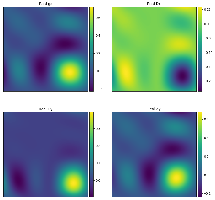
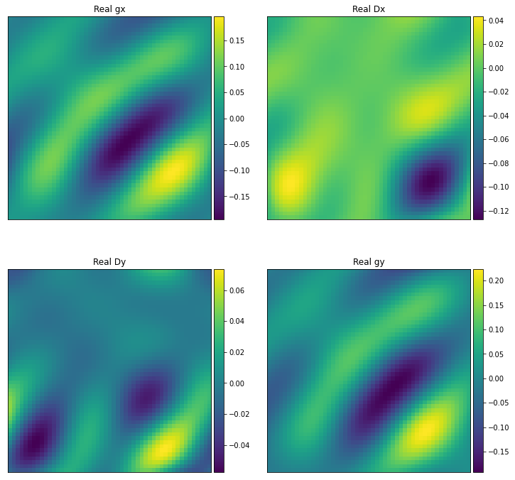
If you want to look at your outputs, you can run the notebook located at cmake_testing/primary_beam_cuda/run_header_setup_and_plots.ipynb. Along with setting up the az/za coords used in the testing, it will generate a number of plots. It will plot the real gains and leakages of the MWA analytic beam (e.g. jones_MWA_analy_gains_nside101_t00_f200.000MHz.png):

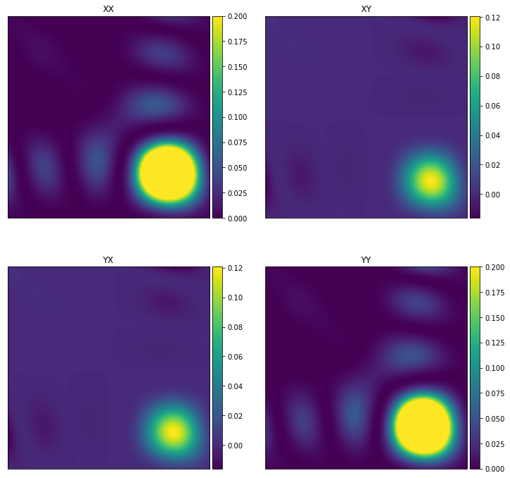
as well as the linear Stokes polarisations (e.g. linear_pol_MWA_analy_gains_nside101_t00_f200.000MHz.png):

test_run_hyperbeam.c

This calls primary_beam_cuda::test_run_hyperbeam_cuda, which calls primary_beam_cuda::run_hyperbeam_cuda, which is a wrapper around mwa_hyperbeam to calculate the MWA FEE beam.

The MWA beam pointing direction on the sky is controlled by a set of 16 delays. In these tests, three different delays settings are tested at 50MHz, 150MHz, and 250MHz (a total of nine tests). Each test is run with ~10,000 sky directions, for two time steps (with identical az/za coords; in reality, those change with time) and three fine frequency channels. The fine frequency channels all lie with a 1.28MHz frequency resolution of the FEE beam model, so should come out identically. Test with two times and three freqs to check our indexing is working correctly. For each combination of settings, the beam gains output by test_run_hyperbeam.c are compared to those stored in the header test_run_hyperbeam.h.

The header test_run_hyperbeam.h is generated by the notebook run_header_setup_and_plots.ipynb, which uses the Python implementation of mwa_hyperbeam to calculate expected outcomes.

All delay and frequency combinations are run with both parallactic angle rotation applied and not. Both the FLOAT and DOUBLE codes are checked to match the Python version of mwa_hyperbeam to a tolerance of 1e-6 (only one library is linked from mwa_hyperbeam so the accuracy is the same). Again, running run_header_setup_and_plots.ipynb will produce plots.

When applying parallactic angle rotation, and latitude is required, which can change with time (happens when precessing the array back to J2000 for every time step). To check things are working, two time steps with different latitudes are called. To accomodate all these variables, a smaller number of directions on the sky are used to save space / computation.

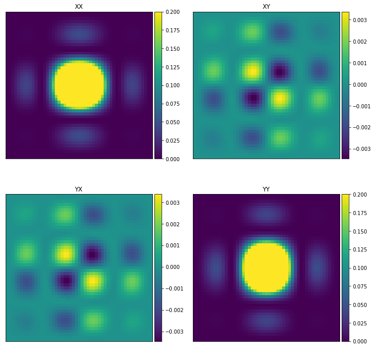
First, an example zenith pointing in Stokes linear (linear_pol_hyperbeam_rot_zenith_gains_nside51_t00_f200.000MHz.png):

and the equivalent hyperbeam outputs to the pointing used above in test_MWA_analytic.c for comparison:

as well as the linear Stokes polarisations (e.g. linear_pol_MWA_analy_gains_nside101_t00_f200.000MHz.png):

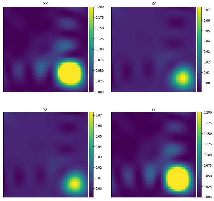
which shows qualitatively the Stokes polarisation responses off zenith are broadly similar between the analytic and FEE beams, but the mutual coupling does modify the response. The gains and leakages are strikingly different, but this is in part because the analytic beam is purely real, whereas the FEE model is complex.

test_run_hyperbeam_interp.c

This calls primary_beam_cuda::test_run_hyperbeam_cuda, which calls primary_beam_cuda::run_hyperbeam_cuda, which is a wrapper around mwa_hyperbeam to calculate the MWA FEE beam. Unlike test_run_hyperbeam.c however, we used the interpolated hdf5 file which has a higher frequency resolution, to give a smooth response as a function of frequency.

Three tests are run, with three different pointings and three different frequency ranges. The output values are then tested against values output by python version of hyperdrive, with the outputs tested to a tolerance of 1e-10.

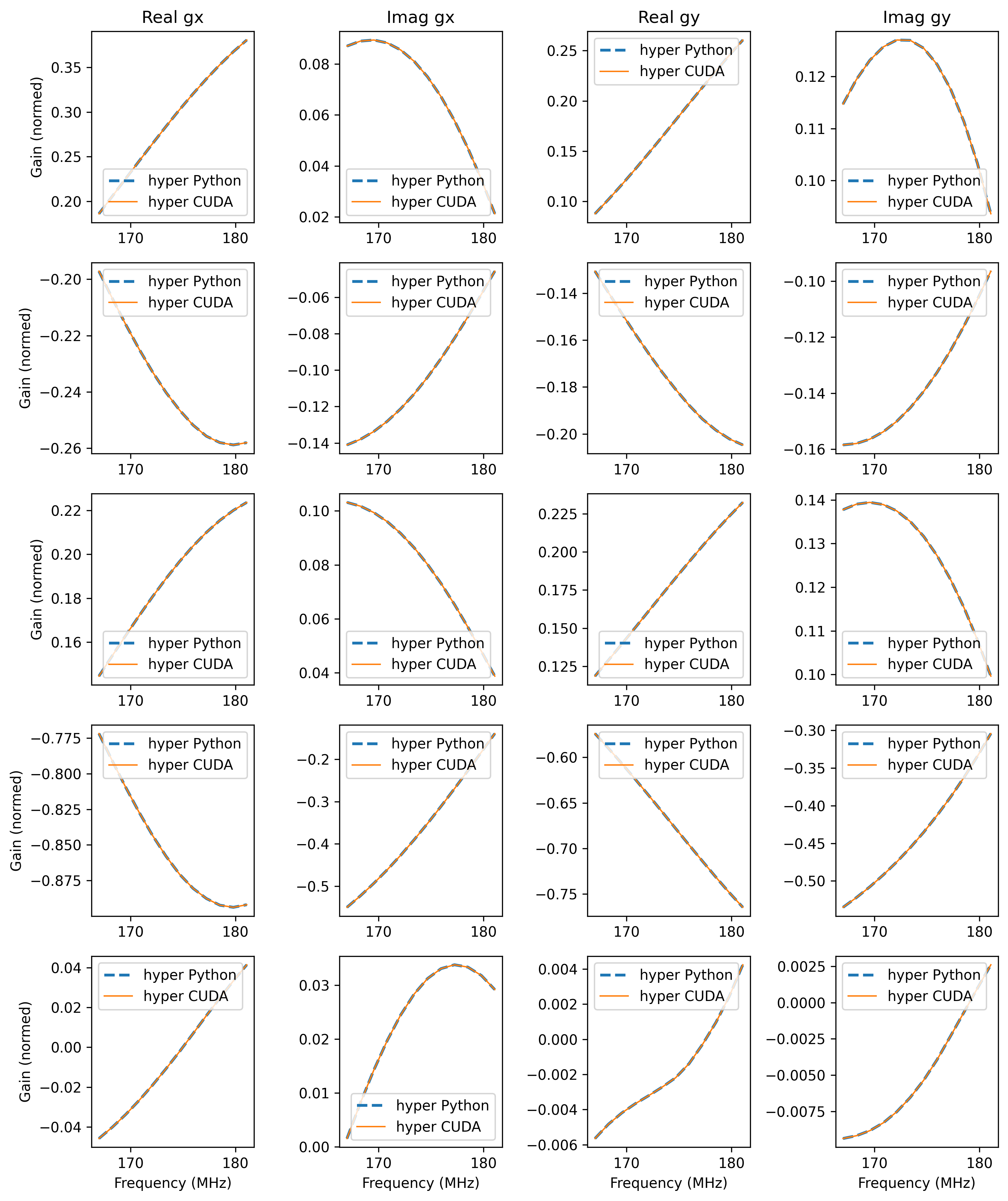
Only five coordinate directions are tested, as the accuracy of the beam across the sky is tested for many many directions by test_run_hyperbeam.c, which is using the same code. This test is really check that the correct frequencies are called, and subsequently mapped correctly. Again, we can plot the outputs using run_header_setup_and_plots.ipynb,which yields plots like offzen1_freqs2.png, plotting the gains and leakages as a function of frequency, for five different direction on the sky (each a different row):